Physikalische Grundlagen der Nuklearmedizin/ Methoden der 3D-Visualisierung
Einleitung
[Bearbeiten]Dies ist ein in der Entwicklung befindliches Kapitel des Wikibooks Physikalische Grundlagen der Nuklearmedizin
Dreidimensionale Visualisierungsmethoden werden verwendet um Reihen Tomographischer Schnitte in eine Form zu bringen, die oft leichter zu interpretieren ist als die Schnitte selbst. Dieses Kapitel gibt eine Übersicht über die wichtigsten Visualisierungstechniken, die in der Nuklearmedizin verwendet werden. Wir beginnen mit der Zusammenfügung von zweidimensionaler axialer Abbildungen und wenden uns danach dreidimensionalen Darstellungsmethoden zu.
Die folgenden Abbildungen werden uns bei dieser Aufgabe nützlich sein. Sie bestehen aus einer SPECT Lungenventilationsstudie, dargestellt auf der linken Seite, einer SPECT Lungendurchblutungsuntersuchung in der Mitte und ein CT Pulmonales Angiogram (CTPA) von selben Patienten auf der rechten Seite.
 |
 |
 |
Wir werden diese Bilder an verschiedenen Stellen in diesem Kapitel einsetzen und Beispiele angeben, die uns helfen werden das Wesentliche der Techniken mit denen wir uns beschäftigen darzustellen. We'll use these image sets at various stages in this chapter so as to provide examples which will help with demonstrating the essence of the techniques we'll consider. Acquisition factors for the image sets include 128 x 128 pixel slices each of thickness 4.8 mm for the SPECT studies and 512 x 512 pixel contiguous slices of thickness 1.5 mm for the axial images reconstructed from the CTPA helical scan. In addition, the lung-perfusion scan was acquired immediately following the ventilation scan, so that residual activity from the latter is present in the former at a level of about 20%.
Its helpful, before proceeding, to consider the axial slices, be they SPECT or CT, stacked one behind the other, as illustrated below:

Notice that the figure illustrates each image as a thin slice when the data represents in reality a slice wide enough to fill the gap between it and the next slice, so that the image data can be considered to be a matrix of volume elements - called voxels for short.
A convention applied in medical imaging is to display axial image stacks with the axes oriented as shown in the following figure:

So the left side of an axial scan represents the patient's right side viewed from below, with their anterior surface at the top of the image. A modificiation of a little ditty by Spike Milligan might help you remember this perspective:
You're likely to find that its a good idea to experience the real thing when reading this chapter so as to help overcome the abstract nature of many of the topics we'll encounter, as well as the limitations of using a 2D medium (i.e. this webpage) to communicate 3D visualization concepts. Numerous open source 3D programs and image libraries are available via the World Wide Web. The software used to generate images in this chapter, for instance, includes OsiriX (MacOS X only), Madena and ImageJ (multi-platform).
Axial Projection
[Bearbeiten]The first technique we'll consider is a relatively simple one called Axial Projection. It involves integrating a number of axial images to display a composite which presents a three-dimensional impression of that volume of image data. The technique is sometimes referred to as Thick Slab or Z-Projection.
The figure below illustrates the outcome of a range of z-projection methods, with a single slice shown in the bottom right hand corner for reference purposes. The first image in the top left shows the result of summing 16 slices, and the other two images on that row show the results of computing the mean and median of these slices.

The first two images in the second row show the result of what are called a Maximum Intensity Projection (MIP) and a Minimum Intensity Projection (MinIP), respectively. A MIP evaluates each voxel along each line of voxels through the volume to determine the maximum voxel value and forms an image using the values so determined for each line. A MinIP uses the minimum voxel values, as illustrated in the following figure:

Volume rendered projections are shown in the first two images along the bottom row of our collection of example axial projections. This image compositing method involves applying an opacity function to the voxel data as well as a recursive addition of the resulting data. An equation of the form:
where
- An = (α).(Voxel Value of voxel, n),
- Bn = (1-α).(Voxel Value of voxel, n-1), and
- α = opacity, in the range 0 (i.e. fully transparent) to 1 (i.e. fully opaque),
is applied to each line of voxels as illustrated in the following figure:

The figure shows the line of voxels we've used previously with an opacity table in the top right corner. The opacity function shown is one where a zero opacity is applied to voxel values below a threshold level, a linear increase in opacity is applied to an intermediate range of voxel values and maximum opacity applied to high voxel values. The opacity table is somewhat like the look-up table used for greyscale windowing which we've described earlier, with the function applied to the opacity of voxel values instead of to their grey levels. Note that more complex opacity tables to the one used in our figure above can be also applied, e.g. logarithmic and exponential functions.
The bottom half of the figure shows the steps involved in calculating the volume rendered value of the composited voxel. Voxel values are shown on the top row with opacity values, derived from a crude opacity table, for each voxel shown on the second row. The third, fourth and fifth rows detail the values of A, B and C, calculated using our volume rendering equation above. The final voxel value is obtained by summing the bottom row, and normalizing the result to, say, a 256 level grey scale.
The outcome of this form of processing is the generation of an image which includes visual depth cues on the basis that similar voxel values will be displayed with a similar transparency and those closest to the reference slice having a stronger contribution than those from more distal slices. Further, note that all voxel values in each line contribute to the rendered image, in contrast to the limited number of voxels that contribute to a MIP or a MinIP image. A 3D effect results from volume rendering, as illustrated in the images above.
Notice that volume rendering can be applied from distal to proximal slices, as illustrated in our figure, as well as in the opposite direction, i.e. from proximal to distal slices. Hence the terms Volume Rendering Up and Volume Rendering Down used in our set of nine example images above.
The type of axial projection method appropriate to an individual patient study is dependent on the anatomical and/or functional information of relevance to the diagnostic process. Let's take the case of imaging contrast-filled blood vessels, for example, in our nine example images above. Note that a MIP can be used to give a visually-stunning impression of the vessel bed in the patient's lungs. There's little depth information in this projection, however, so that overlapping and underlying vessels can obscure lesions that might be present in blood vessels of interest. The application of this form of axial projection to angiography is therefore limited to studies where vessel overlap isn't an issue. The inclusion of voxel transparency and depth weighting in volume rendered images addresses this limitation of MIP processing.
A final point to note is that this form of image projection can also be applied to multi-planar reconstructions of axial slices, which we'll consider next.....
Multi-Planar Reconstruction
[Bearbeiten]In the simplest case, multi-planar reconstruction (MPR) involves generating perspectives at right angles to a stack of axial slices so that coronal and sagittal images can be generated. We'll start this section by describing these orthogonal projections before considering their synchronized composite display. We'll also describe three variants on this theme: oblique reconstruction, curved reconstruction and integrated three-dimensional presentation.
- Coronal Reconstruction
- Here the image stack is rotated so that the z-axis becomes the vertical and a stack of images is reconstructed using parallel planes of voxels arranged from the patient's anterior to posterior surface, as illustrated in the following figure:

- Example coronal reconstructions from our image sets are shown below:
 |
 |
- Here the reconstructed slices are typically displayed from the patient's anterior to their posterior surface with the patient's head towards the top of the slices and their right hand side on the left of the slices.
- Sagittal Reconstruction
- Sagittal reconstructions are possible through additional rotations of the image stack so that a patient's left-to-right slice sequence can be generated as illustrated in the following figure:

- Example sagittal reconstructions from our image sets are shown below:
- Here the reconstructed slices are typically displayed from the patient's left to right side, with their head towards the top and their anterior surface towards the left of the slices. Note that a right-to-left sagittal stack can also be generated using additional geometric transformation of the data.
- Composite MPR Display
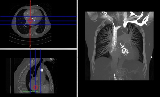
- Coronal and sagittal reconstructions are referred to as Orthogonal MPRs because the perspectives generated are from planes of image data which are at right angles to each other. Composite MPR displays can be generated so that linked cursors or crosshairs can be used to locate a point of interest from all three perspectives, as illustrated in these images:
 |
 |
- This form of image presentation is sometimes referred to as a TCS display - implying the viewing of Transaxial, Coronal and Sagittal slices. It can be combined with the slice projection methods we discussed earlier, as illustrated in the two sets of images below, where the blue lines highlight the limits of the coronal projections:


- Oblique Reconstruction
- Oblique MPRs are possible by defining angled planes through the voxel data , as illustrated in the following figure:

- Here the plane can be defined in, say, the axial images (red line, top left) and a maximum intensity projection (the limits used are highlighted by the blue lines), for example, can be displayed for the reconstructed plane (right). This technique is useful when attempting to generate perspectives in cases where the visualization of three-dimensional structures is complicated by overlapping anatomical detail.
- Curved Reconstruction
- Curved MPRs can be used for the reconstruction of more complex perspectives, as illustrated in the next figure:

- Here a curve (highlighted in green) can been positioned in the axial images (left panel) to define a curved surface which extends through the voxel data in the z-direction, and voxels from this data can be reconstructed into a two-dimensional image (right panel). Note that more complex curves than the one illustrated can be generated so that, for instance, the three-dimensional course of a major blood vessel can be isolated, or CT head scans can be planarized for orthodontic applications.
- 3D Multi-Planar Reconstruction
- A final variant on the MPR theme is the generation of a three-dimensional display showing all three orthogonal projections combined so that a defined point of interest locates the intersection of the planes, as illustrated in the following figure:

- The point of intersection is located for illustrative purposes at the centre of the voxel data in the figure above. It can typically be placed at any point in the 3D data using interactive controls. In addition, the perspective used for the rotating sequence can typically be manipulated interactively to improve the visualization of a region of interest. Note that the image sequence illustrated above is one from a myriad of perspectives that can thus be generated. Note also that slice projections (e.g. MIPs) can be combined with this form of display to provide additional perspectives on a feature of interest.
Maximum Intensity Projection
[Bearbeiten]We've described the maximum intensity projection (MIP) earlier in the context of axial projection, where the maximum voxel value is determined for lines running in parallel through the projected slice thickness. A sequence of such images can be generated when this computation is applied at successive angles around the voxel data. One simple sequence is a rotating one for 360 degrees around the horizontal plane, as illustrated in the left panel of the figure below, where the maximum intensity is projected for every 9 degrees around the patient and the resultant 40 images compiled into a repeating, temporal (e.g. movie) sequence:

Notice that the 3D MIP derives its information from the most attenuating regions of the CT scan (given that the CT-number is directly dependent on the linear attenuation coefficient) and hence portrays bone, contrast media and metal with little information from surrounding, lower attenuating tissues. Notice also that continued viewing of the rotating MIP sequence can generate a disturbing effect where the direction of rotation appears to periodically reverse - which may be an aspect of perceptual oscillation. The perspective MIP, illustrated in the panel on the right in the above figure, can reduce this limitation by providing spatial cues which can be used to guide continued visual inspection.
Perspective projections can be generated by changing from the parallel lines used to generate the parallel projections to lines of voxels which diverge from an apparent point behind the volume at a distance such that the viewer of the display can visualize closer features of the image data as relatively larger than deeper features - see the following figure:

Volume Rendering
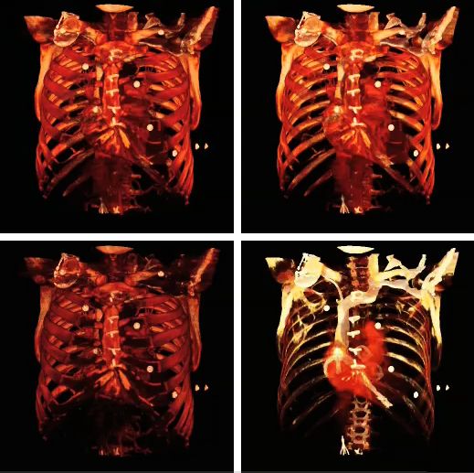
[Bearbeiten]Volume rendering can be applied to the voxel data in the successive rotation manner described for MIPs above, as illustrated by the results in the following figure:

Note that the volume rendering can be contrast enhanced so as to threshold, for instance, through the voxel values to eliminate low attenuating surfaces, as illustrated in the following figure:

Note also that the colour look-up table (CLUT) can be varied to highlight features of particular interest, as shown in the set of images below:

The influence of the opacity table is illustrated in the following example images:

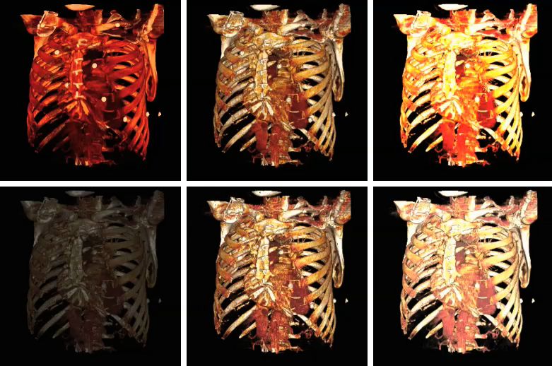
and the influence on volume rendering of various shading settings is shown below:

The shading settings used for the above images are as follows:
| Image | Ambient Coefficient | Diffuse Coefficient | Specular Coefficient | Specular Power |
|---|---|---|---|---|
| Top Left | ||||
| Top Middle | ||||
| Top Right | ||||
| Bottom Left | ||||
| Bottom Middle | ||||
| Bottom Right |
A final feature to note about volume rendering is that 3D editting techniques can be applied so as to exclude unwanted features from the computations and to expose internal structure. This is illustrated in the following figure, where planes of an orthogonal frame can be moved to crop the voxel data from six directions.

Surface Rendering
[Bearbeiten]Surface rendering is also referred to as Shaded Surface Display (SSD) and involves generating surfaces from regions with similar voxel values in the 3D data as illustrated by the SPECT lung-perfusion scan shown in the left panel below:

The process involves the display of surfaces which might potentially exist within the 3D voxel data on the basis that the edges of objects can be expected to have similar voxel values. One approach is to use a grey-level thresholding technique where voxels are extracted once a threshold value is encountered in the line of the projection - see the following diagram. Triangles are then used to tesselate the extracted voxels, as shown in the right panel of the figure above - and the triangles are filled using a constant value with shading applied on the basis of simulating the effects of a fixed virtual light source - as shown in the left panel above.

An opacity table can be applied to the results so that surfaces from internal features can also be visualized. As an example, two surfaces have been identified in the following image from the CT scan where voxel values from bone surfaces are coded in an opaque yellow colour and tissue surfaces in a transparent shade of red.

A second example of using an opacity table is shown in the following figure. Here, axial CT data from the patient's airways have been segmented using a region growth technique and the result processed using surface rendering, with full opacity as shown in the left panel and with a reduced opacity (30%) as shown in the right panel:

Notice that internal features of each lung can be discerned when the opacity is reduced. Notice also that continued viewing of this type of transparency display can generate apparent reversal of the image rotation, similar to that noted for the 3D MIPs above. One method of overcoming this type of problem is to segment each lung, for instance. and to blend the results, as illustrated in the following figure:

subFusion Processing
[Bearbeiten]We'll conclude this chapter by considering an application of 3D visualization which integrates many of the image processing techniques we've described in this wikibook. We'll use the two SPECT scans, from a patient's lung-ventilation (V) and lung-perfusion (Q) studies, in an attempt to visualize any mismatch(es) characteristic of pulmonary embolism (PE). The application we'll consider is called subFusion Processing because it involves both image subtraction and image fusion techniques.
Note again that the SPECT studies were generated using a swamping technique where the perfusion scan was acquired immediately following the ventilation scan using an administered activity which generated a relative count rate of about 5:1 between scans. The first image processing step therefore is to correct the perfusion scan for the background ventilation activity.
Since the ventilation tracer in this case was administered using a aerosol, we can assume for simplicity that its biodistribution is reasonably identical in the two scans. Further, since the scans were acquired about 15 minutes apart using the 99mTc radioisotope, we can assume a neglegible effect from radioactive decay. We can simply therefore subtract the ventilation stack from the perfusion stack, on the basis of these assumptions, to isolate what we'll call the "pure perfusion" scan.
The second step is to normalize the two scans by multiplying the ventilation stack by a factor such that the mean counts (for example) in the two stacks are similar.
- We can now compare apples with apples!
Since a PE mismatch is likely to arise from regions of the lungs which contain counts in the ventilation scan and are relatively bereft of such counts in the perfusion scan, we can subtract the "pure perfusion" stack from the ventilation stack, as a third image processing step, to isolate any such differences as positively-valued features.
The final image processing step is to volume render this difference stack along with the "pure perfusion" scan and to blend the results, as illustrated in the following image:

The steps involved are outlined in the following diagram. Note that minor processes, such as CLUT selection, relative opacity adjustment and contrast enhancement are omitted from this diagram for the sake of simplicity. Note also that an image registration step may need inclusion at the beginning of the procedure in cases where patient movement occurs between the two SPECT acquisitions.

A final point to note is the larger appearance of the patient's lungs in the segmented CTPA images relative to the SPECT images. This arises because the CTPA study was acquired using a single breath-hold and the SPECT studies with the patient breathing quietly over the period of gamma camera rotation. The spatial registration of the three sets of images is therefore not possible directly, and would require the application of spatial warping and other techniques which, unfortunately, are beyond the scope of our treatment here.


