Epsilon-delta definition of continuity

Among the sequence criteria, the epsilon-delta criterion is another way to define the continuity of functions. This criterion describes the feature of continuous functions, that sufficiently small changes of the argument cause arbitrarily small changes of the function value.

Motivation

In the beginning of this chapter, we learned that continuity of a function may - by a simple intuition - be considered as an absence of jumps. So if we are at an argument where continuity holds, the function values will change arbitrarily little, when we wiggle around the argument by a sufficiently small amount. So $f(x)\approx f(x_0)$, for $x$ in the vicinity of $x_0$ . The function values $f(x)$ may therefore be useful to approximate $f(x_0)$ .

Continuity when approximating function values

If a function has no jumps, we may approximate its function values by other nearby values . For this approximation, and hence also for proofs of continuity, we will use the epsilon-delta criterion for continuity. So how will such an approximation look in a practical situation?

Suppose, we make an experiment that includes measuring the air temperature as a function of time. Let $f$ be the function describing the temperature. So $f(x)$ is the temperature at time $x$. Now, suppose there is a technical problem, so we have no data for $f(x_0)$ - or we simply did not measure $f$ at exactly this point of time. However, we would like to approximate the function value $f(x_0)$ as precisely as we can:

At time x_0 , the temperature is f(x_0)

Suppose, a technical issue prevented the measurement of $f(x_0)$ . Since the temperature changes continuously in time - and especially there is no jump at $x_0$ - we may instead use a temperature value measured at a time close to $x_0$ . So, let us approximate the value $f(x_0)$ by taking a temperature $f(x)$ with $x$ close to $x_0$ . That means, $f(x)$ is an approximation for $f(x_0)$. How close must $x$ come to $x_0$ in order to obtain a given approximation precision?

Suppose that for the evaluation of the temperature at a later time $x$ , the maximal error shall be $ϵ=\mathrm{0,1}{}^{\mathrm{\circ }}\mathrm{C}$ . So considering the following figure, the measured temperature should be in the grey region . Those are all temperatures with function values between $f(x_0)-ϵ$ and $f(x_0)+ϵ$ , i.e. inside the open interval $(f(x_0)-ϵ,f(x_0)+ϵ)$ :

Epsilon-region around the function value f(x_0)

In this graphic, we may see that there is a region around $x_0$ , where function values differ by less than $ϵ$ from $f(x_0)$ . So in fact, there is a time difference $\delta$, such that all function values are inside the interval $(x_0-\delta ,x_0+\delta )$ highlighted in grey:

Delta-region around x_0, where all function values lie in an epsilon-region around f(x_0)

Therefore, we may indeed approximate the missing data point $f(x_0)$ sufficiently well (meaning with a maximal error of $ϵ$) . This is done by taking a time $x$ differing from $x_0$ by less than $\delta$ and then, the error of $f(x)$ in approximating $f(x_0)$ will be smaller than the desired maximal error $ϵ$. So $f(x)$ will be the approximation for $f(x_0)$ .

Conclusion: There is a $\delta >0$, such that the difference $|f(x)-f(x_0)|$ is smaller than $ϵ$ for all $|x-x_0|$ smaller than $\delta$ . I.e. $|x-x_0|<\delta ⟹|f(x)-f(x_0)|<ϵ$

Increasing approximation precision

What will happen, if we need to know the temperature value to a higher precision due to increased requirements in the evaluation of the experiment? For instance, if the required maximal temperature error is set to ${ϵ}_2=\mathrm{0,05}{}^{\mathrm{\circ }}\mathrm{C}$ instead of $ϵ=\mathrm{0,1}{}^{\mathrm{\circ }}\mathrm{C}$ ?

Small epsilon-interval around the function value f(x_0)

In that case, thare is an interval around $x_0$, where function values do not deviate by more than ${ϵ}_2$ from $f(x_0)$ . Mathematically speaking, there a ${\delta }_2>0$ exists, such that $f(x)$ differs by a maximum amount of ${ϵ}_2$ from $f(x_0)$ , if there is $|x-x_0|<{\delta }_2$ :

Small delta-interval around x_0, where all function values are in a small interval around f(x_0)

No matter how small we choose $ϵ$ , thanks to the continuous temperature dependence, we may always find a $\delta >0$ , such that $f(x)$ differs at most by $ϵ$ from $f(x_0)$ , whenever $x$ is closer to $x_0$ than $\delta$ . We keep in mind:

No matter which maximal error $ϵ>0$ is required, there is always an interval around $x_0$ , which is $(x_0-\delta ,x_0+\delta )$ with size $\delta >0$, where all approximated function values $f(x)$ deviate by less than $ϵ$ from the function value $f(x_0)$ to be approximated.

This holds true , since the function $f$ does not have a jump at $x_0$ . In other words, since $f$ is continuous at $x_0$. Even beyond that, we may always infer from the above characteristic that there is no jump in the graph of $f$ at $x_0$. Therefore, we may use it as a formal definition for continuity. As mathematicians frequently use the variables $ϵ$ and $\delta$ when describing this characteristic, it is also called epsilon-delta-criterion for continuity.

Epsilon-delta-criterion for continuity

Why does the epsilon-delta-criterion hold if and only if the graph of the function does not have a jump at some argument (i.e. it is continuous there)? The temperature example allows us to intuitively verify, that the epsilon-delta-criterion is satisfied for continuous functions. But will the epsilon-delta-criterion be violated, when a function has a jump at some argument? To answer this question, let us assume that the temperature as a function of time has a jump at some $x_0$:

Function with a jump at x_0

Let $ϵ$ be a given maximal error that is smaller than the jump:

Epsilon-interval with an epsilon smaller than the jump

In that case, we may not choose a $\delta$-interval $(x_0-\delta ,x_0+\delta )$ around $x_0$, where all function values have a deviation lower than $ϵ$ from $f(x_0)$. If we, for instance, choose the following $\delta$, then there certainly is an $x$ between $x_0-\delta$ and $x_0+\delta$ with a function value differing by more than $ϵ$ from $f(x_0)$:

x is inside a delta-interval around x_0, but its function value f(x) has a distance larger than epsilon to f(x_0)

When choosing a smaller ${\delta }_2$, we will find an $x\in (x_0-{\delta }_2,x_0+{\delta }_2)$ with $|f(x)-f(x_0)|\ge ϵ$, as well:

x is situated in a delta-interval around x_0, but f(x) differs by more than epsilon from f(x_0)

No matter how small we choose $\delta$, there will always be an argument $x$ with a distance of less than $\delta$ to $x_0$, such that the function value $f(x)$ differs by more than $ϵ$ from $f(x_0)$. So we have seen that in an intuitive example, the epsilon-delta-criterion is not satisfied, if the function has a jump. Therefore, the epsilon-delta-criterion characterizes whether the graph of the function has a jump at the considered argument $x_0$ or not. That means, we may consider it as a definition of continuity. Since this criterion only uses mathematically well-defined terms, it may be used not just as an intuitive, but also as a formal definition.

Definition

Epsilon-Delta criterion for continuity

The $ϵ$-$\delta$ definition of continuity at an argument $x_0$ inside the domain of definition is the following:

Definition (Epsilon-Delta-definition of continuity)

A function $f:D\to ℝ$ with $D\subseteq ℝ$ is continuous at $x_0\in D$, if and only if for any $ϵ>0$ there is a $\delta >0$ , such that $|f(x)-f(x_0)|<ϵ$ holds for all $x\in D$ with $|x-x_0|<\delta$ . Written in mathematical symbols, that means $f$ is continuous at $x_0\in D$ if and only if

$\mathrm{\forall }ϵ>0\mathrm{\exists }\delta >0\mathrm{\forall }x\in D:|x-x_0|<\delta ⟹|f(x)-f(x_0)|<ϵ$

Explanation of the quantifier notation:

$\begin{array}{c}\begin{array}{c}\underset{\text{For all }ϵ>0}{\underbrace{\mathrm{\forall }ϵ>0}}\underset{\text{ there is a }\delta >0}{\underbrace{\mathrm{\exists }\delta >0}}\underset{\text{, such that for all }x\in D}{\underbrace{\mathrm{\forall }x\in D}}\\ \underset{\text{ with distance to }{x}_0\text{ smaller than }\delta }{\underbrace{|x-x_0|<\delta }}\underset{\text{ there is}}{\underbrace{⟹}}\underset{\text{, such that the distance of }f(x)\text{ to }f(x_0)\text{ is smaller than }ϵ}{\underbrace{|f(x)-f(x_0)|<ϵ}}\end{array}\end{array}$

The above definition describes continuity at a certain point (argument). An entire function $f:D\to ℝ$ is called continuous, when it is continuous - according to the epsilon-delta criterion - at each of its arguments in the domain of definition.

Derivation of the Epsilon-Delta criterion for discontinuity

We may also obtain a criterion of discontinuity by simply negating the above definition. Negating mathematical propositions has already been treated in chapter „Aussagen negieren“ . While doing so, an all quantifier $\mathrm{\forall }$ gets transformed into an existential quantifier $\mathrm{\exists }$ and vice versa. Concerning inner implication, we have to keep in mind that the negation of $A⟹B$ is equivalent to $A\wedge \mathrm{\neg }B$ . Negating the epsilon-delta criterion of discontinuity, we obtain:

$\begin{array}{c}\begin{array}{ccccccc}& \mathrm{\neg }(\mathrm{\forall }ϵ>0& \mathrm{\exists }\delta >0& \mathrm{\forall }x\in D:& |x-x_0|<\delta & ⟹& |f(x)-f(x_0)|<ϵ)\\ ⟺& \mathrm{\exists }ϵ>0& \mathrm{\neg }(\mathrm{\exists }\delta >0& \mathrm{\forall }x\in D:& |x-x_0|<\delta & ⟹& |f(x)-f(x_0)|<ϵ)\\ ⟺& \mathrm{\exists }ϵ>0& \mathrm{\forall }\delta >0& \mathrm{\neg }(\mathrm{\forall }x\in D:& |x-x_0|<\delta & ⟹& |f(x)-f(x_0)|<ϵ)\\ ⟺& \mathrm{\exists }ϵ>0& \mathrm{\forall }\delta >0& \mathrm{\exists }x\in D:& \mathrm{\neg }(|x-x_0|<\delta & ⟹& |f(x)-f(x_0)|<ϵ)\\ ⟺& \mathrm{\exists }ϵ>0& \mathrm{\forall }\delta >0& \mathrm{\exists }x\in D:& |x-x_0|<\delta & \wedge & \mathrm{\neg }(|f(x)-f(x_0)|<ϵ)\\ ⟺& \mathrm{\exists }ϵ>0& \mathrm{\forall }\delta >0& \mathrm{\exists }x\in D:& |x-x_0|<\delta & \wedge & |f(x)-f(x_0)|\ge ϵ\end{array}\end{array}$

This gets us the negation of continuity (i.e. discontinuity):

$\mathrm{\exists }ϵ>0\mathrm{\forall }\delta >0\mathrm{\exists }x\in D:|x-x_0|<\delta \wedge |f(x)-f(x_0)|\ge ϵ$

Epsilon-Delta criterion for discontinuity

Definition (Epsilon-Delta definition of discontinuity)

A function $f:D\to ℝ$ with $D\subseteq ℝ$ is discontinuous at $x_0\in D$, if and only if there is an $ϵ>0$ , such that for all $\delta >0$ a $x\in D$ with $|x-x_0|<\delta$ and $|f(x)-f(x_0)|\ge ϵ$ exists. Mathematically written, $f$ is discontinuous at $x_0\in D$ iff

$\mathrm{\exists }ϵ>0\mathrm{\forall }\delta >0\mathrm{\exists }x\in D:|x-x_0|<\delta \wedge |f(x)-f(x_0)|\ge ϵ$

Explanation of the quantifier notation:

$\begin{array}{c}\begin{array}{c}\underset{\text{There is a }ϵ>0,}{\underbrace{\mathrm{\exists }ϵ>0}}\underset{\text{ such that for all }\delta >0}{\underbrace{\mathrm{\forall }\delta >0}}\underset{\text{ there is an }x\in D}{\underbrace{\mathrm{\exists }x\in D}}\\ \underset{\text{ with distance to }{x}_0\text{ smaller than }\delta }{\underbrace{|x-x_0|<\delta }}\underset{\text{ and}}{\underbrace{\wedge }}\underset{\text{the distance of }f(x)\text{ to }f(x_0)\text{ is bigger (or equal) }ϵ}{\underbrace{|f(x)-f(x_0)|\ge ϵ}}\end{array}\end{array}$

Further explanations considering the Epsilon-Delta criterion

The inequality $|x-x_0|<\delta$ means that the distance between $x$ and $x_0$ is smaller than $\delta$ . Analogously, $|f(x)-f(x_0)|<ϵ$ tells us that the distance between $f(x)$ and $f(x_0)$ is smaller than $ϵ$ . Therefor, the implication $|x-x_0|<\delta ⟹|f(x)-f(x_0)|<ϵ$ just says that whenever $f(x)$ and $f(x_0)$ are closer together than $ϵ$ , then we know that the distance between $x$ and $x_0$ before applying the function must have been smaller than $\delta$ . Thus we may interpret the epsilon-delta criterion in the following way:

No matter how small we set the maximal distance $ϵ$ between function values $f(x)$ , there will always be a $\delta >0$, such that $f(x)$ and $f(x_0)$ (after being mapped) are closer together than $ϵ$ , whenever $x$ is closer to $x_0$ than $\delta$ .

For continuous functions, we can control the error $f(x)$ to be lower than $ϵ$ by keeping the error in the argument sufficiently small (smaller than $\delta$). Finding a $\delta$ means answering the question: How low does my initial error in the argument have to be in order to get a final error smaller than $ϵ$ . This may get interesting when doing numerical calculations or measurements. Imagine, you are measuring some $x_0$ and then using it to compute $f(x_0)$ where $f$ is a continuous function. The epsilon-delta criterion allows you to find the maximal error $\delta$ in $x$ (i.e. $|x-x_0|<\delta$), which guarantees that the final error $|f(x)-f(x_0)|$ will be smaller than $ϵ$.

A $\delta$ may only be found if small changes around the argument $x_0$ also cause small changes around the function value $f(x_0)$ . Hence, concerning functions continuous at $x_0$ , there has to be:

$x\approx x_0⟹f(x)\approx f(x_0)$

I.e.: whenever $x$ is sufficiently close to $x_0$ , then $f(x)$ is approximately $f(x_0)$. This may also be described using the notion of an $ϵ$-neighborhood:

For every $ϵ$-neighborhood $(f(x_0)-ϵ,f(x_0)+ϵ)$ around $f(x_0)$ - no matter how small it may be - there is always a $\delta$-neighborhood $(x_0-\delta ,x_0+\delta )$ around $x_0$, whose function values are all mapped into the $ϵ$-neighborhood.

In topology, this description using neighborhoods will be generalized to a topological definition of continuity.

Visualization of the Epsilon-Delta criterion

Description of continuity using the graph

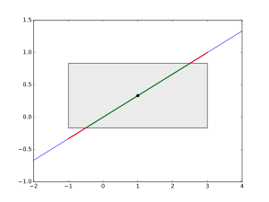
The epsilon-delta criterion may nicely be visualized by taking a look at the graph of a funtion. Let's start by getting a picture of the implication $|x-x_0|<\delta ⟹|f(x)-f(x_0)|<ϵ$. This means, the distance between $f(x)$ and $f(x_0)$ is smaller than epsilon, whenever $x$ is closer to $x_0$ than $\delta$ . So for $x\in (x_0-\delta ,x_0+\delta )$, there is $f(x)\in (f(x_0)-ϵ,f(x_0)+ϵ)$. Hence, the point $(x,f(x))$ has to be inside the rectangle $(x_0-\delta ,x_0+\delta )\times (f(x_0)-ϵ,f(x_0)+ϵ)$ . This is a rectangle with width $2\delta$ and height $2ϵ$ centered at $(x_0,f(x_0))$:

The 2epsilon-2delta-rectangle

We will call this the $2ϵ$-$2\delta$-rectangle and only consider its interior. That means, the boundary does not belong to the rectangle. Following the epsilon-delta criterion, the implication $|x-x_0|<\delta ⟹|f(x)-f(x_0)|<ϵ$ has to be fulfilled for all arguments $x$ . Thus, all points making up the graph of $f$ restricted to arguments inside the interval $(x_0-\delta ,x_0+\delta )$ (in the interior of the $2ϵ$-$2\delta$-rectangle, which is marked green) must never be above or below the rectangle (the red area):

The 2epsilon-2delta-rectangle with allowed and forbidden areas

So graphically, we may describe the epsilon-delta criterion as follows:

For all rectangle heights $ϵ>0$ , there is a sufficiently small rectangle width $\delta >0$, such that the graph of $f$ restricted to $(x_0-\delta ,x_0+\delta )$ (i.e. the width of the rectangle) is entirely inside the green interior of the $2ϵ$-$2\delta$-rectangle, and never in the red above or below area.

Example of a continuous function

For an example, consider the function $f:ℝ\to ℝ:x\mapsto \frac{1}{3}x$ . This fucntion is continuous everywhere - and hence also at the argument $x_0=1$. There is $f(x_0)=f(1)=\frac{1}{3}\cdot 1=\frac{1}{3}$. At first, consider a maximal final error of $ϵ=1$ around $f(x_0)$. With $\delta =2$ , we can find a $\delta >0$, such that the graph of $f$ is entirely situated inside the interior of the $2ϵ$-$2\delta$-rectangle:

Visualization of epsilon-delta continuity

But not only for $ϵ=1$, but for any $ϵ>0$ we may find a $\delta >0$ , such that the graph of $f$ is situated entirely inside the respective $2ϵ$-$2\delta$-rectangle:

• 
  For $ϵ=\frac{1}{2}$ , one can choose $\delta =1$ and the graph is in the interior of the $2ϵ$-$2\delta$-rectangle.
• 
  In case $ϵ=\frac{1}{3}$, the width $\delta =\frac{3}{4}$ will be small enough to get the graph into the $2ϵ$-$2\delta$-rectangle.

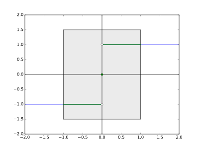
Example for a discontinuous function

What happens if the function is discontinuous? Let's take the signum function $\mathrm{sgn}$, which is discontinuous at 0:

$\mathrm{sgn}:ℝ\to ℝ:x\mapsto \{\begin{array}{cc}1& x>0\\ 0& x=0\\ -1& x<0\end{array}$

And here is its graph:

Graph of the signum function

The graph intuitively allows to recognize that at $x_0=0$ , there certainly is a discontinuity. And we may see this using the rectangle visualization, as well. When choosing a rectangle height $ϵ$, smaller than the jump height (i.e. $ϵ<1$), then there is no $\delta$, such that the graph can be fitted entirely inside the $2ϵ$-$2\delta$-rectangle. For instance if $ϵ=\frac{1}{2}$ , then for any $\delta$ - no matter how small - there will always be function values above or below the $2ϵ$-$2\delta$-rectangle. In fact, this apples to all values except for $f(0)=0$:

• 
  For $ϵ=\frac{1}{2}$ and $\delta =2$ , the signum function has values above or below the $2ϵ$-$2\delta$-rectangle (colored in red).
• 
  For $\delta =\frac{1}{2}$ we will find points in the graph above or below the $2ϵ$-$2\delta$-rectangle, as well.

Dependence of delta or epsilon choice

Continuity

How does the choice of $\delta >0$ depend on $x_0$ and $ϵ$? Suppose, an arbitrary $ϵ>0$ is given in order to check continuity of $f$. Now, we need to find a rectangle width $\delta >0$ , such that the restriction of the graph of $f$ to arguments inside the interval $(x_0-\delta ,x_0+\delta )$ entirely fits into the epsilon-tube $(f(x_0)-ϵ,f(x_0)+ϵ)$ . This of course requires choosing $\delta$sufficiently small. When $\delta$ is too large, there may be an argument $x$ in $(x_0-\delta ,x_0+\delta )$, where $f(x)$ has escaped the tube, i.e. it has a distance to $f(x_0)$ larger than $ϵ$ :

• 
  If for a given $ϵ$ , the respective $\delta$ is chosen too large, then there may be function values above or below the $2ϵ$-$2\delta$-rectangle (marked red, here).
• 
  By contrast, if $\delta$ is re-scaled to be sufficiently small, the graph entirely fits into the $2ϵ$-$2\delta$-rectangle.

How small $\delta$ has to be chosen, will depend on three factors: The function $f$, the given $ϵ$ and the argument $x_0$. Depending on the function slope, a different $\delta$ chosen (steep functions require a smaller $\delta$). Furthermore, for a smaller $ϵ$ we also have to choose a smaller $\delta$ . The following diagrams illustrate this: Here, a quadratic function is plotted, which is continuous at $x_0=1$ . For a smaller $ϵ$ , we also need to choose a smaller $\delta$ :

Dependence of δ on ε: In general, δ has to be chosen smaller as ε shrinks.

The choice of $\delta$ will depend on the argument $x_0$, as well. The more a function changes in the neighborhood of a certain point (i.e. it is steep around it), the smaller we have to choose $\delta$ . The following graphic demonstrates this: The $\delta$-value proposed there is sufficiently small at $x_0$ , but too large at $x_1$ :

The value for delta is sufficiently small for x_0, but too large for x_1.

In the vicinity of $x_1$ , the function $f$ has a higher slope compared to $x_0$. Hence, we need to choose a smaller $\delta$ at $x_1$ . Let us denote the $\delta$-values at $x_0$ and $x_1$ correspondingly by ${\delta }_0$ and ${\delta }_1$ - and choose ${\delta }_1$ to be smaller:

Both interval widths delta_1 and delta_2 are small enough for the given epsilon.

So, we have just seen that the choice of $\delta$ depends on the function $f$ to be considered, as well as the argument $x_0$ and the given $ϵ$ .

Discontinuity

For a discontinuity proof, the relations between the variables will interchange. This relates back to the interchange of the quantifiers under negation of propositions. In order to show discontinuity, we need to find an $ϵ>0$ small enough, such that for no $\delta >0$ the graph of $f$ fits entirely into the $2ϵ$-$2\delta$-rectangle. In particular, if the discontinuity is caused by a jump, then $ϵ$ must be chosen smaller than the jump height. For $ϵ$ too large, there might be a $\delta$, such that $f$ does fit into the $2ϵ$-$2\delta$-rectangle:

• 
  Choosing $ϵ$ too lage for the signum function, we get a $\delta$, such that the graph entirely fits into the $2ϵ$-$2\delta$-rectangle.
• 
  If $ϵ$ is chosen small enough, then for any $\delta >0$ there will be function values above or below the $2ϵ$-$2\delta$-retangle.

Which $ϵ$has to be chosen again depends on the function around $x_0$ . After $ϵ$ has been chosen, an arbitrary $\delta >0$ will be considered. Then, an $x$ between $x_0-\delta$ and $x_0+\delta$ has to be found, such that $f(x)$ has a distance larger than (or equal to) $ϵ$ to $f(x_0)$ . That means, the point $(x,f(x))$ has to be situated above or below the $2ϵ$-$2\delta$-rectangle. Which $x$ has to be chosen depends on a varety of parameters: the chosen $ϵ$ and the arbitrarily given $\delta$, the discontinuity and the behavior of the function around it.

Example problems

Continuity

Exercise (Continuity of a linear function)

Prove that a linear function $f:ℝ\to ℝ$ with $f(x)=\frac{1}{3}x$ is continuous.

How to get to the proof? (Continuity of a linear function)

Graph of a function $f:ℝ\to ℝ$ with $f(x)=\frac{1}{3}x$. Considering the graph , we see that this function is continuous everywhere.

To actually prove continuity of $f$ , we need to check continuity at any argument $x_0\in ℝ$ . So let $x_0$ be an arbitrary real number. Now, choose any arbitrary maximal error $ϵ>0$ . Our task is now to find a sufficiently small $\delta >0$ , such that $|f(x)-f(x_0)|<ϵ$ for all arguments $x$ with $|x-x_0|<\delta$ . Let us take a closer look at the inequality $|f(x)-f(x_0)|<ϵ$ :

$\begin{array}{c}\begin{array}{ccc}& |f(x)-f(x_0)|& <ϵ\\ ⟺& |\frac{1}{3}x-\frac{1}{3}{x}_0|& <ϵ\\ ⟺& |\frac{1}{3}(x-x_0)|& <ϵ\\ ⟺& \frac{1}{3}|x-x_0|& <ϵ\end{array}\end{array}$

That means, $\frac{1}{3}|x-x_0|<ϵ$ has to be fulfilled for all $x$ with $|x-x_0|<\delta$ . How to choose $\delta$ , such that $|x-x_0|<\delta$ implies $\frac{1}{3}|x-x_0|<ϵ$ ?

We use that the inequality $\frac{1}{3}|x-x_0|<ϵ$ contains the distance $|x-x_0|$ . As $|x-x_0|<\delta$ we know that this distance is smaller than $\delta$ . This can be plugged into the inequality $\frac{1}{3}|x-x_0|$ :

$\frac{1}{3}|x-x_0|\stackrel{|x-x_0|<\delta }{<}\frac{1}{3}\delta$

If $\delta$ is now chosen such that $\frac{1}{3}\delta \le ϵ$ , then $\frac{1}{3}|x-x_0|<\frac{1}{3}\delta$ will yield the inequality $\frac{1}{3}|x-x_0|<ϵ$ which we wanted to show. The smallness condition for $\delta$ can now simply be found by resolving $\frac{1}{3}\delta \le ϵ$ for $\delta$:

$\frac{1}{3}\delta \le ϵ⟺\delta \le 3ϵ$

Any $\delta$ satisfying $0<\delta \le 3ϵ$ could be used for the proof. For instance, we may use $\delta =3ϵ$. As we now found a suitable $\delta$, we can finally conduct the proof:

Proof (Continuity of a linear function)

Let $f:ℝ\to ℝ$ with $f(x)=\frac{1}{3}x$ and let $x_0\in ℝ$ be arbitrary. In addition, consider any $ϵ>0$ to be given. We choose $\delta =3ϵ$. Let $x\in ℝ$ with $|x-x_0|<\delta$. There is:

$\begin{array}{cc}|f(x)-f(x_0)|& =|\frac{1}{3}x-\frac{1}{3}{x}_0|\\ & =|\frac{1}{3}(x-x_0)|\\ & =\frac{1}{3}|x-x_0|\\ & \downarrow |x-x_0|<\delta \\ & <\frac{1}{3}\delta \\ & \downarrow \delta =3ϵ\\ & \le \frac{1}{3}(3ϵ)=ϵ\end{array}$

This shows $|f(x)-f(x_0)|<ϵ$, and establishes continuity of $f$ at $x_0$ by means of the epsilon-delta criterion. Since $x_0\in ℝ$ was chosen to be arbitrary, we also know that the entire function $f$ is continuous.

Discontinuity

Exercise (Discontinuity of the signum function)

Prove that the signum function is $\mathrm{sgn}:ℝ\to ℝ$ is discontinuous:

$\mathrm{sgn}(x)=\{\begin{array}{cc}1& x>0\\ 0& x=0\\ -1& x<0\end{array}$

How to get to the proof? (Discontinuity of the signum function)

In order to prove discontinuity of the entire function, we just have to find one single argument where it is discontinuous. Considering the graph of $\mathrm{sgn}$ , we can already guess, which argument this may be:

Graph of the signum function

The function has a jump at $x_0=0$ . So we expect it to be discontinuous, there. It remains to choose an $ϵ>0$ that makes it impossible to find a $\delta >0$ , that makes the function fit into the $2ϵ$-$2\delta$-rectangle. This is done by setting $ϵ$ smaller than the jump height $1$ - for instance $ϵ=\frac{1}{2}$. For that $ϵ$, no matter how $\delta >0$ is given, there will be function values above or below the $2ϵ$-$2\delta$-rectangle.

So let $\delta >0$ be arbitrary. We need to show that there is an $x$ with $|x-x_0|<\delta$ but $|f(x)-f(x_0)|\ge ϵ$ . Let us take a look at the inequality $|x-x_0|<\delta$ :

$|x-x_0|<\delta \stackrel{x_0=0}{⟺}|x|<\delta$

This inequality classifies all $x$ that can be used for the proof. The particular $x$ we choose has to fulfill $|f(x)-f(x_0)|\ge ϵ$ :

$\begin{array}{c}\begin{array}{ccc}& |f(x)-f(x_0)|& \ge ϵ\\ ⟺& |\mathrm{sgn}(x)-\mathrm{sgn}(x_0)|& \ge \frac{1}{2}\\ ⟺& |\mathrm{sgn}(x)-\mathrm{sgn}(0)|& \ge \frac{1}{2}\\ ⟺& |\mathrm{sgn}(x)|& \ge \frac{1}{2}\end{array}\end{array}$

So our $x$ needs to fulfill both $|x|<\delta$ and $|\mathrm{sgn}(x)|\ge \frac{1}{2}$ . The second inequality $|\mathrm{sgn}(x)|\ge \frac{1}{2}$ may be achieved quite easily: For any $x\ne 0$ , the value $\mathrm{sgn}(x)$ is either $1$ or $-1$. So $x\ne 0$ does always fulfill $|\mathrm{sgn}(x)|=1\ge \frac{1}{2}$.

Now we need to fulfill the first inequality $|x|<\delta$. From the second inequality, we have just concluded $x\ne 0$ . This is particularly true for all $x$ with $0<x<\delta$ . Therefore, we choos $x$ to be somewhere between $0$ and $\delta$ , for instance $x=\frac{0+\delta }{2}=\frac{\delta }{2}$.

The following figure shows that this is a sensible choice. The $2ϵ$-$2\delta$-rectangle with $ϵ=\frac{1}{2}$ and $\delta =\frac{1}{2}$ is drawn here. All points above or below that rectangle are marked red. These are exactly all $x$ inside the interval $(-\delta ,\delta )$ excluding $0$. Our chosen $x=\frac{\delta }{2}$ (red dot) is situated directly in the middle of the red part of the graph above the rectangle:

At x=δ/2, the graph is above the 2ϵ-2δ-rectangle

So choosing $x=\frac{\delta }{2}$ is enough to complete the proof:

Proof (Discontinuity of the signum function)

We set $x_0=0$ (this is where $f$ is discontinuous). In addition, we choose $ϵ=\frac{1}{2}$. Let $\delta >0$ be arbitrary. For that given $\delta$, we choose $x=\frac{\delta }{2}$. Now, on one hand there is:

$\begin{array}{c}\begin{array}{ccc}& \frac{1}{2}& <1\\ ⟹& \frac{1}{2}\delta & <\delta \\ ⟹& \left|\frac{1}{2}\delta \right|& <\delta \\ ⟹& |\frac{1}{2}\delta -0|& <\delta \\ ⟹& |x-x_0|& <\delta \end{array}\end{array}$

But on the other hand:

$\begin{array}{cc}|f(x)-f(x_0)|& =|\mathrm{sgn}(x)-\mathrm{sgn}(x_0)|\\ & =|\mathrm{sgn}\left(\frac{\delta }{2}\right)-\mathrm{sgn}(0)|\\ & =|1-0|\\ & =1\\ & \ge \frac{1}{2}=ϵ\end{array}$

So indeed, $\mathrm{sgn}$ is discontinuous at $x_0=0$ . Hence, the function $\mathrm{sgn}$ is discontinuous itself.

Relation to the sequence criterion

Now, we have two definitions of continuity: the epsilon-delta and the sequence criterion. In order to show that both definitions describe the same concept, we have to prove their equivalence. If the sequence criterion is fulfilled, it must imply that the epsilon-delta criterion holds and vice versa.

Epsilon-delta criterion implies sequence criterion

Theorem (The epsilon-delta criterion implies the sequence criterion)

Let $f:D\to ℝ$ with $D\subseteq ℝ$ be any function. If this function satisfies the epsilon-dela criterion at $x_0\in D$ , then the sequence criterion is fulfilled at $x_0$ , as well.

How to get to the proof? (The epsilon-delta criterion implies the sequence criterion)

Let us assume that the function $f:D\to ℝ$ satisfies the epsilon-delta criterion at $x_0\in D$ . That means:

For every $ϵ>0$ , there is a $\delta >0$ such that $|f(x)-f(x_0)|<ϵ$ for all $x\in D$ with $|x-x_0|<\delta$ .

We now want to prove that the sequence criterion is satisfied, as well. So we have to show that for any sequence of arguments $(x_n{)}_{n\in \mathbb{N}}$ converging to $x_0$ , there also has to be $\underset{n\to \mathrm{\infty }}{lim}f(x_n)=f(x_0)$ . We therefor consider an arbitrary sequence of arguments $(x_n{)}_{n\in \mathbb{N}}$ in the domain $x_n\in D$ with $\underset{n\to \mathrm{\infty }}{lim}{x}_n=x_0$. Our job is to show that the sequence of function values ${(f(x_n))}_{n\in \mathbb{N}}$ converges to $f(x_0)$ . So by the definition of convergence:

For any $ϵ>0$ there has to be an $N\in \mathbb{N}$ such that $|f(x_n)-f(x_0)|<ϵ$ for all $n\ge N$.

Let $ϵ>0$ be arbitrary. We have to find a suitable $N\in \mathbb{N}$ with $|f(x_n)-f(x_0)|<ϵ$ for all sequence elements beyond that $N$ , i.e. $n\ge N$ . The inequality $|f(x_n)-f(x_0)|<ϵ$ seems familiar, recalling the epsilon-delta criterion. The only difference is that the argument $x$ is replaced by a sequence element $x_n$ - so we consider a special case for $x$ . Let us apply the epsilon-delta criterion to that special case, with our arbitrarily chosen $ϵ$ being given:

There is a $\delta >0$, such that $|f(x_n)-f(x_0)|<ϵ$ for all sequence elements $x_n$ fulfilling $|x_n-x_0|<\delta$ .

Our goal is coming closer. Whenever a sequence element $x_n$ is close to $x_0$ with $|x_n-x_0|<\delta$ , it will satisfy the inequality which we want to show, namely $|f(x_n)-f(x_0)|<ϵ$. It remains to choose an $N\in \mathbb{N}$, where this is the case for all sequence elements beyond $x_N$ . The convergence $\underset{n\to \mathrm{\infty }}{lim}{x}_n=x_0$ implies that $|x_n-x_0|$ gets arbitrarily small. So by the definition of continuity, we may find an $\tilde{N}\in \mathbb{N}$, with $|x_n-x_0|<\delta$ for all $n\ge \tilde{N}$ . This $\tilde{N}$ now plays the role of our $N$. If there is $n\ge N=\tilde{N}$, it follows that $|x_n-x_0|<\delta$ and hence $|f(x_n)-f(x_0)|<ϵ$ by the epsilon-delta criterion. In fact, any $N\ge \tilde{N}$ will do the job. We now conclude our considerations and write down the proof:

Proof (The epsilon-delta criterion implies the sequence criterion)

Let $f:D\to ℝ$ e a function satisfying the epsilon-delta criterion at $x_0\in D$ . Let $(x_n{)}_{n\in \mathbb{N}}$ be a sequence inside the domain of definition, i.e. $x_n\in D$ for all $n\in \mathbb{N}$ coverging as $\underset{n\to \mathrm{\infty }}{lim}{x}_n=x_0$. We would like to show that for any given $ϵ>0$ there exists an $N\in \mathbb{N}$ , such that $|f(x_n)-f(x_0)|<ϵ$ holds for all $n\ge N$ .

So let $ϵ>0$ be given. Following the epsilon-delta criterion, there is a $\delta >0$, with $|f(x)-f(x_0)|<ϵ$ for all $x\in D$ close to $x_0$ , i.e. $|x-x_0|<\delta$ . As $(x_n{)}_{n\in \mathbb{N}}$ converges to $x_0$ , we may find an $N\in \mathbb{N}$ with $|x_n-x_0|<\delta$ for all $n\ge N$ .

Now, let $n\ge N$ be arbitrary. Hence, $|x_n-x_0|<\delta$. The epsilon-delta criterion now implies $|f(x_n)-f(x_0)|<ϵ$. This proves $\underset{n\to \mathrm{\infty }}{lim}f(x_n)=f(x_0)$ and therefore establishes the epsilon-delta criterion.

Sequence criterion implies epsilon-delta criterion

Theorem (The sequence criterion implies the epsilon-delta criterion)

Let $f:D\to ℝ$ with $D\subseteq ℝ$ be a function. If $f$ satisfies the sequence criterion at $x_0\in D$ , then the epsilon-delta criterion is fulfilled there, as well.

How to get to the proof? (The sequence criterion implies the epsilon-delta criterion)

We need to show that the following implication holds:

$f\text{ satisfies the sequence criterion in }{x}_0\in D⟹f\text{ satisfies the epsilon-delta criterion in }{x}_0\in D$

This time, we do not show the implication directly, but using a contraposition. So we will prove the following implication (which is equivalent to the first one):

$\mathrm{\neg }(f\text{ satisfies the epsilon-delta criterion in }{x}_0\in D)⟹\mathrm{\neg }(f\text{ satisfies the sequence criterion in }{x}_0\in D)$

Or in other words:

$f\text{ violates the epsilon-delta criterion in }{x}_0\in D⟹f\text{ violates the sequence criterion in }{x}_0\in D$

So let $f:D\to ℝ$ be a function that violates the epsilon-delta criterion at $x_0\in D$ . Hence, $f$ fulfills the discontinuity version of the epsilon-delta criterion at $x_0$. We can find an $ϵ>0$,such that for any $\delta >0$ there is a $x\in D$ with $|x-x_0|<\delta$ but $|f(x)-f(x_0)|\ge ϵ$ . It is our job now to prove, that the sequence criterion is violated, as well. This requires choosing a sequence of aguments $(x_n{)}_{n\in \mathbb{N}}$ , converging as $\underset{n\to \mathrm{\infty }}{lim}{x}_n=x_0$ but $\underset{n\to \mathrm{\infty }}{lim}f(x_n)\ne f(x_0)$ .

This choice will be done exploiting the discontinuity version of the epsilon-delta criterion. That version provides us with an $ϵ>0$ , where $|f(x)-f(x_0)|\ge ϵ$ holds (so continuity is violated) for certain arguments $x$ . We will now construct our sequence exclusively out of those certain $x$ . This will automatically get us $\underset{n\to \mathrm{\infty }}{lim}f(x_n)\ne f(x_0)$.

So how to find a suitable sequence of arguments $(x_n{)}_{n\in \mathbb{N}}$, converging to $x_0$ ? The answer is: by choosing a null sequence $({\delta }_n{)}_{n\in \mathbb{N}}$. Practically, this is done as follows: we set ${\delta }_n=\frac{1}{n}$ . For any ${\delta }_n$ , we take one of the certain $x$ for $\delta ={\delta }_n$ as our argument $x_n$ . Then, $|x_n-x_0|<{\delta }_n$ but also $|f(x_n)-f(x_0)|\ge ϵ$. These $x_n$ make up the desired sequence $(x_n{)}_{n\in \mathbb{N}}$. On one hand, there is $|x_n-x_0|<{\delta }_n$ and as $\underset{n\to \mathrm{\infty }}{lim}{\delta }_n=0$ , the convergence $\underset{n\to \mathrm{\infty }}{lim}{x}_n=x_0$ holds. But on the other hand $|f(x_n)-f(x_0)|\ge ϵ$ , so the sequence of function values ${(f(x_n))}_{n\in \mathbb{N}}$ does not converge to $f(x_0)$ . Let us put these thoughts together in a single proof:

Proof (The sequence criterion implies the epsilon-delta criterion)

We establish the theorem by contraposition. It needs to be shown that a function $f:D\to ℝ$ violating the epsilon-delta criterion at $x_0\in D$ also violates the sequence criterion at $x_0$ . So let $f:D\to ℝ$ with $D\subseteq ℝ$ be a function violating the epsilon-delta criterion at $x_0\in D$ . Hence, there is an $ϵ>0$, such that for all $\delta >0$ an $x\in D$ exists with $|x-x_0|<\delta$ but $|f(x)-f(x_0)|\ge ϵ$ .

So for any ${\delta }_n=\frac{1}{n}$ , there is an $x_n\in D$ with $|x_n-x_0|<{\delta }_n$ but $|f(x_n)-f(x_0)|\ge ϵ$. The inequality $|x_n-x_0|<{\delta }_n$ can also be written $x_0-{\delta }_n\le x_n\le x_0+{\delta }_n$. As $\underset{n\to \mathrm{\infty }}{lim}{\delta }_n=0$ , there is both $\underset{n\to \mathrm{\infty }}{lim}{x}_0-{\delta }_n=x_0$ and $\underset{n\to \mathrm{\infty }}{lim}{x}_0+{\delta }_n=x_0$. Thus, by the sandwich theorem, the sequence $(x_n{)}_{n\in \mathbb{N}}$ converges to $x_0$.

But since $|f(x_n)-f(x_0)|\ge ϵ$ for all $n\in \mathbb{N}$ , the sequence ${(f(x_n))}_{n\in \mathbb{N}}$ can not converge to $f(x_0)$ . Therefore, the sequence criterion is violated at $x_0$ for the function $f$ : We have found a sequence of arguments $(x_n{)}_{n\in \mathbb{N}}$ with $\underset{n\to \mathrm{\infty }}{lim}{x}_n=x_0$ but $\underset{n\to \mathrm{\infty }}{lim}f(x_n)\ne f(x_0)$.

Exercises

Quadratic function

Exercise (Continuity of the quadratic function)

Prove that the function $f:ℝ\to ℝ$ with $f(x)=x^2$ is continuous.

How to get to the proof? (Continuity of the quadratic function)

For this proof, we need to show that the square function is continuous at any argument $x_0\in ℝ$ . Using the proof structure for the epsilon-delta criterion, we are given an arbitrary $ϵ>0$ . Our job is to find a suitable $\delta >0$ , such that the inequality $|f(x)-f(x_0)|<ϵ$ holds for all $|x-x_0|<\delta$.

In order to find a suitable $\delta$ , we plug in the definition of the function $f(x)=x^2$ into the expression $|f(x)-f(x_0)|$ which shall be smaller than $ϵ$:

$|f(x)-f(x_0)|=|x^2-x_0^2|$

The expression $|x-x_0|$ may easily be controlled by $\delta$. Hence, it makes sense to construct an upper estimate for $|x^2-x_0^2|$ which includes $|x-x_0|$ and a constant. The factor $|x-x_0|$ appears if we perform a factorization using the third binomial formula:

$|x^2-x_0^2|=|x+x_0||x-x_0|$

The requirement $|x-x_0|<\delta$ allows for an upper estimate of our expression:

$|x+x_0||x-x_0|<|x+x_0|\cdot \delta$

The $\delta$ we are looking for may only depend on $ϵ$ and $x_0$ . So the dependence on $x$ in the factor $|x+x_0|\cdot \delta$ is still a problem. We resolve it by making a further upper estimate for the factor $|x-x_0|$ . We will use a simple, but widely applied "trick" for that: A $x_0$ is subtracted and then added again at another place (so we are effectively adding a 0) , such that the expression $x-x_0$ appears:

$|x+x_0|\cdot \delta =|x\underset{=0}{\underbrace{-x_0+x_0}}+x_0|\cdot \delta =|x-x_0+2x_0|\cdot \delta$

The absolute $|x-x_0|$ is obtained using the triangle inequality. This absolute $|x-x_0|$ is again bounded from above by $\delta$ :

$|x-x_0+2x_0|\cdot \delta \le (|x-x_0|+|2x_0|)\cdot \delta <(\delta +2|x_0|)\cdot \delta$

So reshaping expressions and applying estimates, we obtain:

$|f(x)-f(x_0)|<(\delta +2|x_0|)\cdot \delta$

With this inequality in hand, we are almost done. If $\delta$ is chosen in a way that $(\delta +2|x_0|)\cdot \delta \le ϵ$ , we will get the final inequality $|f(x)-f(x_0)|<ϵ$ . This $\delta$ is practically found solving the quadratic equation ${\delta }^2+2|x_0|\delta =ϵ$ for $\delta$ . Or even simpler, we may estimate $(\delta +2|x_0|)\cdot \delta$ from above. We use that we may freely impose any condition on $\delta$ . If we, for instance, set $\delta \le 1$, then $\delta +2|x_0|\le 1+2|x_0|$ which simplifies things:

$|f(x)-f(x_0)|<(\underset{\le 1+2|x_0|}{\underbrace{\delta +2|x_0|}})\cdot \delta \le (1+2|x_0|)\cdot \delta$

So $(1+2|x_0|)\cdot \delta \le ϵ$ will also do the job. This inequality can be solved for $\delta$ to get the second condition on $\delta$(the first one was $\delta \le 1$):

$(1+2|x_0|)\cdot \delta \le ϵ⟺\delta \le \frac{ϵ}{1+2|x_0|}$

So any $\delta$ fulfilling both conditions does the job: $\delta \le 1$ and $\delta =\frac{ϵ}{1+2|x_0|}$ have to hold. Ind indeed, both are true for $\delta :=min\{1,\frac{ϵ}{1+2|x_0|}\}$. This choice will be included into the final proof:

Proof (Continuity of the quadratic function)

Let $ϵ>0$ be arbitrary and $\delta :=min\{1,\frac{ϵ}{1+2|x_0|}\}$. If an argument $x$ fulfills $|x-x_0|<\delta$ then:

$\begin{array}{cc}|f(x)-f(x_0)|& =|x^2-x_0^2|\\ & =|x+x_0||x-x_0|\\ & \downarrow |x-x_0|<\delta \\ & <|x+x_0|\cdot \delta \\ & =|x\underset{=0}{\underbrace{-x_0+x_0}}+x_0|\cdot \delta \\ & =|x-x_0+2x_0|\cdot \delta \\ & \le (|x-x_0|+2|x_0|)\cdot \delta \\ & \downarrow |x-x_0|<\delta \\ & <(\delta +2|x_0|)\cdot \delta \\ & \downarrow \delta \le 1\\ & \le (1+2|x_0|)\cdot \delta \\ & \downarrow \delta =\frac{ϵ}{1+2|x_0|}\\ & =(1+2|x_0|)\cdot \frac{ϵ}{1+2|x_0|}\\ & =ϵ\end{array}$

This shows that the square function is continuous by the epsilon-delta criterion.

Concatenated absolute function

Exercise (Example for a proof of continuity)

Prove that the following function is continuous at $x_0=1$:

$f:ℝ\to ℝ:x\mapsto f(x)=5|x^2-2|+3$

How to get to the proof? (Example for a proof of continuity)

We need to show that for each given $ϵ>0$ , there is a $\delta >0$ , such that for all $x\in ℝ$ with $|x-x_0|<\delta$ the inequality $|f(x)-f(x_0)|<ϵ$ holds. In our case, $x_0=1$. So by choosing $|x-1|<\delta$ for $\delta$ small enough, we may control the expression $|x-1|$ . First, let us plug $x_0=1|$ into $|f(x)-f(x_0)|$ in order to simplify the inequality to be shown $|f(x)-f(x_0)|<ϵ$ :

$\begin{array}{cc}|f(x)-f(x_0)|& =|f(x)-f(1)|\\ & =|5\cdot |x^2-2|+3-(5|1^2-2|+3)|\\ & =|5\cdot |x^2-2|-5|\\ & =5\cdot ||x^2-2|-1|\end{array}$

The objective is to "produce" as many expressions $|x-1|$ as possible, since we can control $|x-1|<\delta$. It requires some experience with epsilon-delta proofs in order to "directly see" how this is achieved. First, we need to get rid of the double absolute. This is done using the inequality $||a|-|b||\le |a-b|$ . For instance, we could use the following estimate:

$\begin{array}{cc}|f(x)-f(x_0)|& =\dots \\ & =5\cdot ||x^2-2|-1|\\ & =5\cdot ||x^2-2|-|1||\\ & \downarrow ||a|-|b||\le |a-b|\\ & \le 5\cdot |x^2-2-1|\\ & =5\cdot |x^2-3|\end{array}$

However, this is a bad estimate as the expression $|x^2-3|$ no longer tends to 0 as $x\to 1$ . To resolve this problem, we use $1=|-1|$ before applying the inequality $||a|-|b||\le |a-b|$ :

$\begin{array}{cc}|f(x)-f(x_0)|& =\dots \\ & =5\cdot |x^2-2|-1|\\ & =5\cdot |x^2-2|-|-1||\\ & \downarrow |a-b|\ge ||a|-|b||\\ & \le 5\cdot |x^2-2-(-1)|\\ & =5\cdot |x^2-1|\end{array}$

A factor of $|x-1|$ can be directly extracted out of this with the third binomial fomula:

$\begin{array}{cc}|f(x)-f(x_0)|& =\dots \\ & \le 5\cdot |x^2-1|\\ & =5\cdot |x+1||x-1|\end{array}$

And we can control it by $|x-1|<\delta$:

$\begin{array}{cc}|f(x)-f(x_0)|& =\dots \\ & \le 5\cdot |x^2-1|\\ & =5\cdot |x+1||x-1|\\ & <5\cdot |x+1|\cdot \delta \end{array}$

Now, the required $\delta$ must only depend on $ϵ$ and $x_0$ . Therefore, we have to get rid of the $x$-dependence of $5|x+1|\cdot \delta$. This can be done by finding an upper bound for $5|x+1|$ which does not depend on $x$. As we are free to chose any $\delta$ for our proof, we may also impose any condition to it which helps us with the upper bound. In this case, $\delta \le 1$ turns out to be quite useful. In fact, $\delta \le 2$ or an even higher bound would do this job, as well. What follows from this choice?

As before, there has to be $|x-1|<\delta$. As $\delta \le 1$ , we now have $|x-1|<1$ and as $x\in [1-1;1+1]$ , we obtain $1+x\in [1;3]$ and $|x+1|\le 3$. This is the upper bound we were looking for:

$\begin{array}{cc}|f(x)-f(x_0)|& =\dots \\ & <5\cdot |x+1|\cdot \delta \\ & \downarrow |x+1|\le 3\\ & \le 15\cdot \delta \end{array}$

As we would like to show $|f(x)-f(1)|<ϵ$ , we set $\delta =\frac{ϵ}{15}$. And get that our final inequality holds:

$\begin{array}{cc}|f(x)-f(x_0)|& =\dots \\ & <15\cdot \delta \\ & \le 15\cdot \frac{ϵ}{15}\\ & \le ϵ.\end{array}$

So if the two conditions for $\delta$ are satisfied, we get the final inequality. In fact, both conditions will be satisfied if $\delta =min\{1,\frac{ϵ}{15}\}$, concluding the proof. So let's conclude our ideas and write them down in a proof:

Proof (Example for a proof of continuity)

Let $ϵ>0$ be arbitrary and let $\delta =min\{1,\frac{ϵ}{15}\}$. Further, let $x\in ℝ$ with $|x-1|<\delta$. Then:

Step 1: $|x+1|\le 3$

As $\delta =min\{1,\frac{ϵ}{15}\}$ , there is $\delta \le 1$. Hence $|x-1|\le 1$ and $x\in [1-1;1+1]$. It follows that $1+x\in [1;3]$ and therefore $|x+1|\le 3$.

Step 2: $|f(x)-f(x_0)|<ϵ$

$\begin{array}{cc}|f(x)-f(x_0)|& =|f(x)-f(1)|\\ & =|5\cdot |x^2-2|+3-(5|1^2-2|+3)|\\ & =|5\cdot |x^2-2|-5|\\ & =5\cdot ||x^2-2|-1|\\ & \downarrow 1⟺|-1|\\ & =5\cdot ||x^2-2|-|-1||\\ & \downarrow |a-b|\ge ||a|-|b||\\ & \le 5\cdot |x^2-2-(-1)|\\ & =5\cdot |x^2-1|\\ & \downarrow a^2-b^2=(a+b)(a-b)\\ & =5\cdot (|x+1|\cdot \underset{<\delta }{\underbrace{|x-1|}})\\ & <5\cdot |x+1|\cdot \delta \\ & \downarrow |x+1|\le 3\\ & \le 15\delta \\ & \downarrow \delta =\frac{ϵ}{15}\\ & =15\cdot \frac{ϵ}{15}\\ & \le ϵ\end{array}$

Hence, the function is continuous at $x_0=1$ .

Hyperbola

Exercise (Continuity of the hyperbolic function)

Prove that the function $f:{ℝ}^{+}\to ℝ$ with $f(x)=\frac{1}{x}$ is continuous.

How to get to the proof? (Continuity of the hyperbolic function)

The basic pattern for epsilon-delta proofs is applied here, as well. We would like to show the implication $|x-x_0|<\delta ⟹|f(x)-f(x_0)|<ϵ$ . Forst, let us plug in what we know and reshape our terms a bit until a $|x-x_0|$ appears:

$\begin{array}{cc}|f(x)-f(x_0)|& =|\frac{1}{x}-\frac{1}{x_0}|\\ & =\left|\frac{x-x_0}{x\cdot x_0}\right|\\ & =\frac{|x-x_0|}{|x||x_0|}\\ & =\frac{1}{|x||x_0|}\cdot |x-x_0|\end{array}$

By assumption, there will be $|x-x_0|<\delta$, of which we can make use:

$|f(x)-f(x_0)|=\dots =\frac{1}{|x||x_0|}\cdot |x-x_0|<\frac{1}{|x||x_0|}\cdot \delta$

The choice of $\delta$ may again only depend on $ϵ$ and $x_0$ so we need a smart estimate for $\frac{1}{|x|}$ in order to get rid of the $x$-dependence. To do so, we consider $\delta \le \frac{x_0}{2}$.

Why was $\delta \le \frac{x_0}{2}$ and not $\delta \le 1$ chosen? The explanation is quite simple: We need a $\delta$-neighborhood inside the domain of definition of $f$. If we had simply chosen $\delta \le 1$ , we might have get kicked out of this domain. For instance, in case$x_0=\frac{1}{2}$, the following problem appears:

The biggest $x$-value with $|x-\frac{1}{2}|<1$ is $x_{\mathrm{m}\mathrm{a}\mathrm{x}}=\frac{3}{2}$ and the smallest one is $x_{\mathrm{m}\mathrm{i}\mathrm{n}}=-\frac{1}{2}$. However, $x_{\mathrm{m}\mathrm{i}\mathrm{n}}$ is not inside the domain of definition as $f:{ℝ}^{+}\to ℝ$. In particular, $x=0$ is element of that interval, where $f(x)=\frac{1}{x}$ cannot be defined at all.

A smarter choice for $\delta$, such that the $\delta$-neighborhood doesn't touch the $y$-axis is half of the distance to it, i.e. $\delta \le \frac{x_0}{2}$. A third of this distance or other fractions smaller than 1 would also be possible: $\delta \le \frac{x_0}{3}$, $\delta <\frac{x_0}{20}$ or $\delta <\frac{x_0}{5321}$.

As we chose $\delta \le \frac{x_0}{2}$ and by $|x-x_0|<\delta$ , there is $x\in [\frac{x_0}{2};\frac{3x_0}{2}]$. This allows for an upper bound: $\frac{1}{|x|}\le \frac{2}{|x_0|}$ and we may write:

$\begin{array}{cc}|f(x)-f(x_0)|& =\dots <\frac{1}{|x||x_0|}\cdot \delta \\ & \downarrow \delta =\frac{ϵ\cdot |x_0{|}^2}{2}\\ & \le \frac{2}{|x_0{|}^2}\cdot \delta \end{array}$

So we get the estimate:

$|f(x)-f(x_0)|\le \frac{2}{|x_0{|}^2}\cdot \delta$

Now, we want to prove $|f(x)-f(x_0)|<ϵ$ . Hence we choose $\delta \le \frac{ϵ\cdot |x_0{|}^2}{2}$. Plugging this in, our final inequality $|f(x)-f(x_0)|<ϵ$ will be fulfilled.

So again, we imposed two conditions for $\delta$ : $\delta \le \frac{x_0}{2}$ and $\delta \le \frac{ϵ\cdot |x_0{|}^2}{2}$. Both are fulfilled by $\delta =min\{\frac{x_0}{2},\frac{ϵ\cdot |x_0{|}^2}{2}\}$, which we will use in the proof:

Proof (Continuity of the hyperbolic function)

Let $f:{ℝ}^{+}\to ℝ$ with $f(x)=\frac{1}{x}$ and let $x_0\in {ℝ}^{+}$ be arbitrary. Further, let $ϵ>0$ be arbitrary. We choose $\delta :=min\{\frac{x_0}{2},\frac{ϵ\cdot |x_0{|}^2}{2}\}$. For all $x\in ℝ$ with $|x-x_0|<\delta$ there is:

$\begin{array}{cc}|f(x)-f(x_0)|& =|\frac{1}{x}-\frac{1}{x_0}|\\ & =\left|\frac{x-x_0}{x\cdot x_0}\right|\\ & =\frac{|x-x_0|}{|x||x_0|}\\ & =\frac{1}{|x||x_0|}|x-x_0|\\ & \downarrow \frac{1}{|x|}\le \frac{2}{|x_0|}\\ & \le \frac{2}{|x_0{|}^2}|x-x_0|\\ & \downarrow |x-x_0|<\delta \\ & <\frac{2\delta }{|x_0{|}^2}\\ & \downarrow \delta =\frac{ϵ\cdot |x_0{|}^2}{2}\\ & =\frac{2}{|x_0{|}^2}\cdot \frac{ϵ\cdot |x_0{|}^2}{2}\\ & =ϵ\end{array}$

Hence, the function $f$ is continuous at $x_0$ . And as $x_0$ was chosen to be arbitrary, the whole function $f$ is continuous.

Concatenated square root function

Exercise (Epsilon-Delta proof for the continuity of the Square Root Function)

Show, using the epsilon-delta criterion, that the following function is continuous:

$f:ℝ\to ℝ,x\mapsto \sqrt{5+x^2}$

How to get to the proof? (Epsilon-Delta proof for the continuity of the Square Root Function)

We need to show, that for any given $ϵ>0$ , there is a $\delta >0$ , such that all $x\in ℝ$ with $|x-a|<\delta$ satisfy the inequality $|f(x)-f(a)|<ϵ$ . So let us take a look at the target inequality $|f(x)-f(a)|<ϵ$ and estimate the absolute $|f(x)-f(a)|$ from above. We are able to control the term $|x-a|$ . Therefor, would like to get an upper bound for $|f(x)-f(a)|$ including the expression $|x-a|$ . So we are looking for an inequality of the form

$|f(x)-f(a)|\le K(x,a)\cdot |x-a|$

Here, $K(x,a)$ is some expression depending on $x$ and $a$ . The second factor is smaller than $\delta$ and can be made arbitrarily small by a suitable choice of $\delta$ . Such a bound is constructed as follows:

$\begin{array}{cc}|f(x)-f(a)|& =|\sqrt{5+x^2}-\sqrt{5+a^2}|\\ & \downarrow \text{expand with}|\sqrt{5+x^2}+\sqrt{5+a^2}|\\ & =\frac{|\sqrt{5+x^2}-\sqrt{5+a^2}|\cdot |\sqrt{5+x^2}+\sqrt{5+a^2}|}{|\sqrt{5+x^2}+\sqrt{5+a^2}|}\\ & \downarrow \sqrt{5+x^2}+\sqrt{5+a^2}\ge 0\\ & =\frac{|x^2-a^2|}{\sqrt{5+x^2}+\sqrt{5+a^2}}\\ & =\frac{|x+a|}{\sqrt{5+x^2}+\sqrt{5+a^2}}\cdot |x-a|\\ & \downarrow K(x,a):=\frac{|x+a|}{\sqrt{5+x^2}+\sqrt{5+a^2}}\\ & =K(x,a)\cdot |x-a|\end{array}$

Since $|x-a|<\delta$ , there is:

$|f(x)-f(a)|=K(x,a)\cdot |x-a|<K(x,a)\cdot \delta$

If we now choose $\delta$ small enough, such that $K(x,a)\cdot \delta \le ϵ$ , then we obtain our target inequality $|f(x)-f(a)|\le ϵ$. But $K(x,a)$ still depends on $x$ , so $\delta$ would have to depend on , too - and we required one choice of $\delta$ which is suitable for all $x$ . THerefore, we need to get rid of the $x$-dependence. This is done by an estimate of the first factor, such that our inequality takes the form $K(x,a)\le \tilde{K}(a)$ :

$\begin{array}{cc}K(x,a)& =\frac{|x+a|}{\sqrt{5+x^2}+\sqrt{5+a^2}}\\ & \downarrow \text{triangle inequality}\\ & \le \frac{\left|x\right|}{\sqrt{5+x^2}+\sqrt{5+a^2}}+\frac{\left|a\right|}{\sqrt{5+x^2}+\sqrt{5+a^2}}\\ & \downarrow \frac{a}{b+c}\le \frac{a}{b}\text{ for }a,c\ge 0,b>0\\ & \le \frac{\left|x\right|}{\sqrt{5+x^2}}+\frac{\left|a\right|}{\sqrt{5+a^2}}\\ & \downarrow \frac{|a|}{\sqrt{5+a^2}}\le 1\text{, since }\sqrt{5+a^2}\ge \sqrt{a^2}=|a|\\ & \le 2=:\tilde{K}(a)\end{array}$

We even made $\tilde{K}(a)$ independent of $a$ , which would in fact not have been necessary. So we obtain the following inequality

$|f(x)-f(a)|\le 2\cdot |x-a|<2\cdot \delta$

We need the estimate $2\cdot \delta \le ϵ$, in order to fulfill the target inequality $|f(x)-f(a)|<ϵ$ . The choice of $\delta =\frac{ϵ}{2}$ is sufficient for that. So let us write down the proof:

Proof (Epsilon-Delta proof for the continuity of the Square Root Function)

Let $f:ℝ\to ℝ$ with $f(x)=\sqrt{5+x^2}$. Let $a\in ℝ$ and an arbitrary $ϵ>0$ be given. We choose $\delta =\frac{ϵ}{2}$. For all $x\in ℝ$ with $|x-a|<\delta$ there is:

$\begin{array}{cc}|f(x)-f(a)|& =|\sqrt{5+x^2}-\sqrt{5+a^2}|\\ & =\frac{|\sqrt{5+x^2}-\sqrt{5+a^2}|\cdot |\sqrt{5+x^2}+\sqrt{5+a^2}|}{|\sqrt{5+x^2}+\sqrt{5+a^2}|}\\ & =\frac{|x^2-a^2|}{\sqrt{5+x^2}+\sqrt{5+a^2}}\\ & =\frac{|x+a|}{\sqrt{5+x^2}+\sqrt{5+a^2}}\cdot |x-a|\\ & \le (\frac{\left|x\right|}{\sqrt{5+x^2}+\sqrt{5+a^2}}+\frac{\left|a\right|}{\sqrt{5+x^2}+\sqrt{5+a^2}})\cdot |x-a|\\ & \le (\frac{\left|x\right|}{\sqrt{5+x^2}}+\frac{\left|a\right|}{\sqrt{5+a^2}})\cdot |x-a|\\ & \le (1+1)\cdot |x-a|\\ & \le 2\cdot |x-a|\\ & \downarrow |x-a|<\delta =\frac{ϵ}{2}\\ & <2\cdot \frac{ϵ}{2}=ϵ\end{array}$

Hence, $f$ is a continuous function.

Discontinuity of the topological sine function

Exercise (Discontinuity of the topological sine fucntion)

Prove the discontinuity at $x_0=0$ for the topological sine function:

$f:ℝ\to ℝ:x\mapsto \{\begin{array}{cc}\sin \left(\frac{1}{x}\right)& x\ne 0\\ 0& x=0\end{array}$

How to get to the proof? (Discontinuity of the topological sine fucntion)

In this exercise, discontinuity has to be shown for a given function. This is done by the negation of the epsilon-delta criterion. Our objective is to find both an $ϵ>0$ and an $x\in ℝ$, such that $|x-x_0|<\delta$ and $|f(x)-f(x_0)|\ge ϵ$ . Here, $x$ may be chosen depending on $\delta$ , while $ϵ$ has to be the same for all $\delta >0$ . For a solution, we may proceed as follows

Step 1: Simplify the target inequality

First, we may simplify the two inequalities which have to be fulfilled by plugging in $x_0=0$ and $f(x_0)=0$. We therefore get: $|x|<\delta$ and $|f(x)|\ge ϵ$.

Step 2: Choose a suitable $ϵ>0$

We consider the graph of the function $f$ . It will help us finding the building bricks for our proof:

Graph of the topological sine function

We need to find an $ϵ>0$ , such that there are arguments in each arbitrarily narrow interval $(x_0-\delta ,x_0+\delta )=(-\delta ,\delta )$ whose function values have a distance larger than $ϵ$ from $f(x_0)=f(0)=0$ . Visually, no matter how small the width $\delta$ of the $2ϵ$-$2\delta$-rectangle is chosen, there will always be some points below or above it.

Taking a look at the graph, we see that our function oscillates between $-1$ and $1$ . Hence, $ϵ\le 1$ may be useful. In that case, there will be function values with $|f(x)|\ge 1$ in every arbitrarily small neighborhood around $x_0=0$. We choose $ϵ=\frac{1}{2}$. This is visualized in the following figure:

The topological sine function oscillates between -1 and 1 nea the origin. Hence, in each neighborhood around 0, there will be arguments x , where f(x) has a distance larger than 1/2 to 0.

After $ϵ$ has been chosen, an arbitrary $\delta >0$ will be assumed, for which we need to find a suitable $x$. This is what we will do next.

Step 3: Choice of a suitable $x\in ℝ$

We just set $ϵ=\frac{1}{2}$ . Therefore, $|\sin \left(\frac{1}{x}\right)|\ge \frac{1}{2}$ has to hold. So it would be nice to choose an $x$ with $\sin \left(\frac{1}{x}\right)=1$ . Now, $\sin (a)=1$ is obtained for any $a=\frac{\pi }{2}+2k\pi$ with $k\in \mathbb{Z}$ . The condition for $x$ such that the function gets 1 is therefore:

$\frac{1}{x}=\frac{\pi }{2}+2k\pi ⟺x=\frac{1}{\frac{\pi }{2}+2k\pi }$

So we found several $x$ , where $|f(x)|\ge ϵ$ . Now we only need to select one among them, which satisfies $|x|<\delta$ for the given $\delta$ . Our $x$ depend on $k$ . So we have to select a suitable $k\in \mathbb{Z}$ , where $|x|<\delta$ . To do so, let us plug $x=\frac{1}{\frac{\pi }{2}+2k\pi }$ into this inequality and solve it for $k$ :

$\begin{array}{cc}\left|x\right|<\delta & ⟺\left|\frac{1}{\frac{\pi }{2}+2k\pi }\right|<\delta \\ & ⟺\frac{1}{\frac{\pi }{2}+2k\pi }<\delta \\ & ⟺2k\pi +\frac{\pi }{2}>\frac{1}{\delta }\\ & ⟺2k\pi >\frac{1}{\delta }-\frac{\pi }{2}\\ & ⟺k>\frac{1}{2\pi }(\frac{1}{\delta }-\frac{\pi }{2})\end{array}$

So the condition on $k$ is $k>\frac{1}{2\pi }(\frac{1}{\delta }-\frac{\pi }{2})$. If we choose just any natural number $k$ above this threshold $\frac{1}{2\pi }(\frac{1}{\delta }-\frac{\pi }{2})$ , then $|x|<\delta$ will be fulfilled. Such a $k$ has to exist by Archimedes' axiom (for instance by flooring up the right-hand expression). So let us choose such a $k$ and define $x$ via $x=\frac{1}{\frac{\pi }{2}+2k\pi }$ . This gives us both $|x|<\delta$ and $|f(x)|\ge ϵ$ . So we got all building bricks together, which we will now assemble to a final proof:

Proof (Discontinuity of the topological sine fucntion)

Choose $ϵ=\frac{1}{2}$ and let $\delta >0$ be arbitrary. Choose a natural number $k$ with $k>\frac{1}{2\pi }(\frac{1}{\delta }-\frac{\pi }{2})$. Such a natural number $k$ has to exist by Archimedes' axiom. Further, let $x=\frac{1}{\frac{\pi }{2}+2k\pi }$. Then:

$\begin{array}{cc}k>\frac{1}{2\pi }(\frac{1}{\delta }-\frac{\pi }{2})& ⟹2k\pi >\frac{1}{\delta }-\frac{\pi }{2}\\ & ⟹2k\pi +\frac{\pi }{2}>\frac{1}{\delta }\\ & \downarrow \frac{1}{a}>\frac{1}{b}>0⟺0<a<b\\ & ⟹\frac{1}{\frac{\pi }{2}+2k\pi }<\delta \\ & \downarrow \frac{1}{\frac{\pi }{2}+2k\pi }>0\\ & ⟹\left|\frac{1}{\frac{\pi }{2}+2k\pi }\right|<\delta \\ & \downarrow x=\frac{1}{\frac{\pi }{2}+2k\pi }\\ & ⟹\left|x\right|<\delta \end{array}$

In addition:

$\begin{array}{cc}|f(x)-f(0)|& =|\sin \left(\frac{1}{x}\right)-0|\\ & \downarrow x=\frac{1}{\frac{\pi }{2}+2k\pi }\\ & =|\sin (\frac{\pi }{2}+2k\pi )|\\ & \downarrow \sin (\frac{\pi }{2}+2k\pi )=1\\ & =\left|1\right|\ge \frac{1}{2}=ϵ\end{array}$

Hence, the function is discontinuous at $x_0=0$.