Sinus Hyperbolicus und Kosinus Hyperbolicus – Serlo „Mathe für Nicht-Freaks“

Dieser Abschnitt ist noch im Entstehen und noch nicht offizieller Bestandteil des Buchs. Gib der Autorin oder dem Autor Zeit, den Inhalt anzupassen!

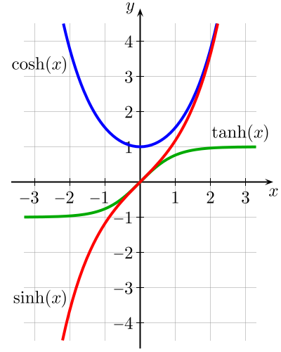Die Hyperbolischen Funktionen - Kosinus Hyperbolikus, Sinus Hyperbolikus und Tangens Hyperbolikus

To-Do:

einleitungstext

Definition von Sinus Hyperbolicus und Kosinus Hyperbolicus

Definition (Sinus Hyperbolicus und Kosinus Hyperbolicus)

Wir definieren die Funktionen $\sinh$ (Sinus Hyperbolicus) und $\cosh$ (Kosinus Hyperbolicus) durch

${\begin{aligned}&\sinh :\mathbb {R} \to \mathbb {R} ,x\mapsto {\frac {1}{2}}(e^{x}-e^{-x})\\[0.3em]&\cosh :\mathbb {R} \to \mathbb {R} ,x\mapsto {\frac {1}{2}}(e^{x}+e^{-x})\end{aligned}}$

Hinweis

Als Merkhilfe für das Vorzeichen: Sinus und Minus reimt sich.

Definition von Tangens Hyperbolicus

Definition (Tangens Hyperbolicus)

Über die Funktionen $\sinh$ und $\cosh$ definieren wir die Funktion $\tanh$ (Tangens Hyperbolicus) durch

${\begin{aligned}&\tanh :\mathbb {R} \to \mathbb {R} ,x\mapsto {\frac {\sinh(x)}{\cosh(x)}}={\frac {e^{x}-e^{-x}}{e^{x}+e^{-x}}}\end{aligned}}$

Eigenschaften der Hyperbolischen Funktionen

Symmetrie

Der Kosinus Hyperbolicus ist symmetrisch zur y-Achse, während Sinus und Tangens Hyperbolicus punktsymmetrisch zum Ursprung sind. Es gilt also:

${\begin{aligned}\cosh(x)&=\cosh(-x)\\\sinh(x)&=-\sinh(-x)\\\tanh(x)&=-\tanh(-x)\\\end{aligned}}$

Man sagt auch $\cosh$ ist eine gerade Funktion, die anderen beiden sind ungerade.

Wir wollen die eben genannten Eigenschaften beweisen:

Beweis

${\begin{aligned}\cosh(-x)&={\frac {1}{2}}\cdot (e^{-x}+e^{-(-x)})={\frac {1}{2}}\cdot (e^{-x}+e^{x})=\cosh(x)\\\sinh(-x)&={\frac {1}{2}}\cdot (e^{-x}-e^{-(-x)})={\frac {1}{2}}\cdot (e^{-x}-e^{x})=-\sinh(x)\\\tanh(-x)&={\frac {\sinh(-x)}{\cosh(-x)}}={\frac {-\sinh(x)}{\cosh(x)}}=-\tanh(x)\end{aligned}}$

Ableitungen

Mit der Definition über die Exponentialfunktion können wir die Ableitungen der Hyperbolischen Funktionen bestimmen.

${\begin{aligned}\cosh(x)^{\prime }&=\sinh(x)\\\sinh(x)^{\prime }&=\cosh(x)\\\tanh(x)^{\prime }&={\frac {1}{\cosh(x)^{2}}}=\tanh(x)^{2}-1\end{aligned}}$

Der Beweis für diese Gleichungen ist im Kapitel Beispiele für Ableitungen zu finden.

Beziehung zwischen den Hyperbolischen Funktionen

Analog zu den Trigonometrischen Funktionen, haben wir eine Beziehung zwischen den Quadraten von $\sinh$ und $\cosh$. Der Unterschied liegt im Vorzeichen.

${\begin{aligned}\cos(x)^{2}&{\color {red}+}\sin(x)^{2}&=1\\\cosh(x)^{2}&{\color {red}-}\sinh(x)^{2}&=1\end{aligned}}$

Beweis

${\begin{aligned}\cosh(x)^{2}-\sinh(x)^{2}&=\left({\frac {e^{x}+e^{-x}}{2}}\right)^{2}-\left({\frac {e^{x}-e^{-x}}{2}}\right)^{2}\\&={\frac {1}{4}}\left[\left(e^{2x}+e^{-2x}+2e^{x}e^{-x}\right)-\left(e^{2x}+e^{-2x}-2e^{x}e^{-x}\right)\right]\\&{\color {OliveGreen}\left\downarrow \ e^{x}e^{-x}=1\right.}\\&={\frac {1}{4}}\cdot 4=1\end{aligned}}$

Asymptotik

Im Grenzwert $x\to \pm \infty$ divergieren $\cosh$ und $\sinh$. Um zu bestimmen ob der Grenzwert $\infty$ oder $-\infty$ ist, setzen wir die Definition durch die Exponentialfunktion.

${\begin{aligned}\lim _{x\to \infty }\cosh(x)&=\lim _{x\to \infty }{\frac {1}{2}}\underbrace {e^{x}} _{\to \infty }+{\frac {1}{2}}\underbrace {e^{-x}} _{\to 0}=\infty \\\lim _{x\to -\infty }\cosh(x)&=\lim _{x\to \infty }{\frac {1}{2}}\underbrace {e^{x}} _{\to 0}+{\frac {1}{2}}\underbrace {e^{-x}} _{\to \infty }=\infty \\\lim _{x\to \infty }\sinh(x)&=\lim _{x\to \infty }{\frac {1}{2}}\underbrace {e^{x}} _{\to \infty }-{\frac {1}{2}}\underbrace {e^{-x}} _{\to 0}=\infty \\\lim _{x\to -\infty }\sinh(x)&=\lim _{x\to \infty }{\frac {1}{2}}\underbrace {e^{x}} _{\to 0}-{\frac {1}{2}}\underbrace {e^{-x}} _{\to \infty }=-\infty \end{aligned}}$

Da $\sinh(ix)=\sin(x)$ und $\cosh(ix)=\cos(x)$ bedeutet das, dass Sinus und Kosinus als Funktionen komplexer Argumente nicht beschränkt sind.

Additionstheoreme

${\begin{aligned}\sinh(x\pm y)&=\sinh x\cosh y\pm \cosh x\sinh y\\\cosh(x\pm y)&=\cosh x\cosh y\pm \sinh x\sinh y\end{aligned}}$

Der Beweis funktioniert völlig analog zu den Trigonometrischen Additionstheoremen.