Deine Meinung zählt – Gestalte unsere Lerninhalte mit!
Wir entwickeln neue, interaktive Formate für die Hochschulmathematik. Nimm dir maximal 15 Minuten Zeit, um an unserer Umfrage
Mit deinem Feedback machen wir die Mathematik für dich und andere Studierende leichter zugänglich!
Dieser Abschnitt ist noch im Entstehen und noch nicht offizieller Bestandteil des Buchs. Gib den Autoren Zeit, den Inhalt anzupassen!
Hauptsatz der Differential- und Integralrechnung [ Bearbeiten ]
Lösung
Lösung Teilaufgabe 2:
1. Abschätzung: Da
t
↦
f
(
t
)
=
1
−
t
8
{\displaystyle t\mapsto f(t)={\sqrt {1-t^{8}}}}
[
0
,
0.5
]
{\displaystyle [0,0.5]}
F
(
0
,
5
)
=
∫
0
0.5
1
−
t
8
d
t
≥
∫
0
0.5
1
−
(
0.5
)
8
d
t
=
[
0.998
t
]
0
0.5
=
0.499
≥
0.496
{\displaystyle F(0,5)=\int _{0}^{0.5}{\sqrt {1-t^{8}}}\mathrm {d} t\geq \int _{0}^{0.5}{\sqrt {1-(0.5)^{8}}}\mathrm {d} t=[0.998t]_{0}^{0.5}=0.499\geq 0.496}
sowie
F
(
0
,
5
)
=
∫
0
0.5
1
−
t
8
d
t
≤
∫
0
0.5
1
−
0
8
d
t
=
[
t
]
0
0.5
=
0.500
{\displaystyle F(0,5)=\int _{0}^{0.5}{\sqrt {1-t^{8}}}\mathrm {d} t\leq \int _{0}^{0.5}{\sqrt {1-0^{8}}}\mathrm {d} t=[t]_{0}^{0.5}=0.500}
2. Abschätzung: Ebenso ist
f
{\displaystyle f}
[
0
,
1
]
{\displaystyle [0,1]}
F
(
1
)
=
∫
0
1
1
−
t
8
d
t
=
∫
0
0.5
1
−
t
8
d
t
+
∫
0.5
0.75
1
−
t
8
d
t
+
∫
0.75
1
1
−
t
8
d
t
≥
∫
0
0.5
1
−
(
0.5
)
8
d
t
⏟
=
0.496
+
∫
0.5
0.75
1
−
(
0.75
)
8
d
t
⏟
=
0.237
+
∫
0.75
1
1
−
1
8
d
t
⏟
=
0
=
0.733
{\displaystyle {\begin{aligned}F(1)&=\int _{0}^{1}{\sqrt {1-t^{8}}}\mathrm {d} t=\int _{0}^{0.5}{\sqrt {1-t^{8}}}\mathrm {d} t+\int _{0.5}^{0.75}{\sqrt {1-t^{8}}}\mathrm {d} t+\int _{0.75}^{1}{\sqrt {1-t^{8}}}\mathrm {d} t\\&\geq \underbrace {\int _{0}^{0.5}{\sqrt {1-(0.5)^{8}}}\mathrm {d} t} _{=0.496}+\underbrace {\int _{0.5}^{0.75}{\sqrt {1-(0.75)^{8}}}\mathrm {d} t} _{=0.237}+\underbrace {\int _{0.75}^{1}{\sqrt {1-1^{8}}}\mathrm {d} t} _{=0}\\&=0.733\end{aligned}}}
Schließlich ist
F
(
1
)
=
∫
0
1
1
−
t
8
d
t
≤
∫
0
1
1
d
t
=
1
{\displaystyle F(1)=\int _{0}^{1}{\sqrt {1-t^{8}}}\mathrm {d} t\leq \int _{0}^{1}{\sqrt {1}}\mathrm {d} t=1}
Aufgabe
Gegeben sei
f
(
x
)
=
∫
1
x
(
t
−
1
)
2
ln
(
t
−
1
)
d
t
{\displaystyle f(x)=\int _{1}^{x}(t-1)^{2}\ln(t-1)\,\mathrm {d} t}
Bestimme den Definitionsbereich von
f
{\displaystyle f}
Untersuche das Monotonieverhalten von
f
{\displaystyle f}
Lösung
Lösung Teilaufgabe 2:
Monotonie: Nach dem Monotoniekriterium ist
f
{\displaystyle f}
f
′
>
0
{\displaystyle f'>0}
f
′
<
0
{\displaystyle f'<0}
Mit dem Hauptsatz der Differential- und Integralrechnung gilt nun für alle
x
∈
[
1
,
∞
[
{\displaystyle x\in [1,\infty [}
f
′
(
x
)
=
(
x
−
1
)
2
ln
(
x
−
1
)
{\displaystyle f'(x)=(x-1)^{2}\ln(x-1)}
Weiter ist für
x
≠
1
{\displaystyle x\neq 1}
(
x
−
1
)
2
⏟
≥
0
ln
(
x
−
1
)
{
>
0
⟺
ln
(
x
−
1
)
>
0
⟺
x
−
1
>
1
⟺
x
>
2
,
<
0
⟺
ln
(
x
−
1
)
<
0
⟺
x
−
1
<
1
⟺
x
<
2
{\displaystyle \underbrace {(x-1)^{2}} _{\geq 0}\ln(x-1){\begin{cases}>0&\iff \ln(x-1)>0\iff x-1>1\iff x>2,\\<0&\iff \ln(x-1)<0\iff x-1<1\iff x<2\end{cases}}}
Damit ist
f
{\displaystyle f}
]
2
,
∞
[
{\displaystyle ]2,\infty [}
]
1
,
2
[
{\displaystyle ]1,2[}
Extrema: Es gilt:
f
′
(
x
)
=
(
x
−
1
)
2
ln
(
x
−
1
)
=
0
⟺
x
=
1
oder
x
=
2
{\displaystyle f'(x)=(x-1)^{2}\ln(x-1)=0\iff x=1{\text{ oder }}x=2}
Da
f
{\displaystyle f}
x
=
1
{\displaystyle x=1}
f
{\displaystyle f}
x
=
2
{\displaystyle x=2}
x
=
2
{\displaystyle x=2}
To-Do:
konvexes und konkaves Verhalten
Lösung
Lösung Teilaufgabe 1:
Zunächst ist
g
(
0
)
=
∫
0
0
2
1
+
t
sin
2
(
t
)
d
t
=
∫
0
0
1
+
t
sin
2
(
t
)
d
t
=
0
{\displaystyle g(0)=\int _{0}^{0^{2}}{\sqrt {1+t\sin ^{2}(t)}}\,\mathrm {d} t=\int _{0}^{0}{\sqrt {1+t\sin ^{2}(t)}}\,\mathrm {d} t=0}
Für den Integranden gilt weiter auf
[
0
,
x
2
]
{\displaystyle [0,x^{2}]}
1
+
t
sin
2
(
t
)
≥
0
{\displaystyle {\sqrt {1+t\sin ^{2}(t)}}\geq 0}
Aus der Monotonie des Integrals folgt für alle
x
∈
R
{\displaystyle x\in \mathbb {R} }
g
(
x
)
=
∫
0
x
2
1
+
t
sin
2
(
t
)
d
t
≥
∫
0
x
2
0
d
t
=
0
=
g
(
0
)
{\displaystyle g(x)=\int _{0}^{x^{2}}{\sqrt {1+t\sin ^{2}(t)}}\,\mathrm {d} t\geq \int _{0}^{x^{2}}0\,\mathrm {d} t=0=g(0)}
Somit hat
g
{\displaystyle g}
Lösung Teilaufgabe 2:
Für die Hilfsfunktion
h
(
y
)
=
∫
0
y
1
+
t
sin
2
(
t
)
d
t
{\displaystyle h(y)=\int _{0}^{y}{\sqrt {1+t\sin ^{2}(t)}}\,\mathrm {d} t}
gilt mit dem Hauptsatz der Differential- und Integralrechnung für alle
y
≥
0
{\displaystyle y\geq 0}
h
′
(
y
)
=
1
+
y
sin
2
(
y
)
{\displaystyle h'(y)={\sqrt {1+y\sin ^{2}(y)}}}
Weiter ist
g
(
x
)
=
h
(
x
2
)
{\displaystyle g(x)=h(x^{2})}
Mit der Kettenregel folgt damit für alle
x
∈
R
{\displaystyle x\in \mathbb {R} }
g
′
(
x
)
=
h
′
(
x
2
)
⋅
2
x
=
1
+
x
2
sin
2
(
x
2
)
⋅
2
x
=
2
x
1
+
x
2
sin
2
(
x
2
)
{\displaystyle g'(x)=h'(x^{2})\cdot 2x={\sqrt {1+x^{2}\sin ^{2}(x^{2})}}\cdot 2x=2x{\sqrt {1+x^{2}\sin ^{2}(x^{2})}}}
Lösung (Substitutionsregel 1)
Teilaufgabe 1:
∫
1
1
+
x
d
x
↓
Substitution
y
=
1
+
x
⟹
d
y
d
x
=
1
⟹
d
x
=
d
y
=
∫
1
y
d
y
↓
Hauptsatz der Differential- und Integralrechnung
=
ln
(
y
)
+
c
↓
Rücksubstitution:
y
=
1
+
x
=
ln
(
1
+
x
)
+
c
{\displaystyle {\begin{aligned}&\int {\frac {1}{1+x}}\,\mathrm {d} x\\[0.5em]&{\color {OliveGreen}\left\downarrow \ {\text{Substitution }}y=1+x\Longrightarrow {\frac {\mathrm {d} y}{\mathrm {d} x}}=1\Longrightarrow \mathrm {d} x=\mathrm {d} y\right.}\\[0.5em]&{}=\int {\frac {1}{y}}\,\mathrm {d} y\\[0.5em]&{\color {OliveGreen}\left\downarrow \ {\text{Hauptsatz der Differential- und Integralrechnung}}\right.}\\[0.5em]&{}=\ln(y)+c\\[0.5em]&{\color {OliveGreen}\left\downarrow \ {\text{Rücksubstitution: }}y=1+x\right.}\\[0.5em]&{}=\ln(1+x)+c\end{aligned}}}
Teilaufgabe 2:
∫
1
1
+
x
2
d
x
↓
Hauptsatz der Differential- und Integralrechnung
=
arctan
(
x
)
+
c
{\displaystyle {\begin{aligned}&\int {\frac {1}{1+x^{2}}}\,\mathrm {d} x\\[0.5em]&{\color {OliveGreen}\left\downarrow \ {\text{Hauptsatz der Differential- und Integralrechnung}}\right.}\\[0.5em]&{}=\arctan(x)+c\end{aligned}}}
Teilaufgabe 3:
∫
x
1
+
x
d
x
=
∫
1
+
x
−
1
1
+
x
d
x
=
∫
(
1
+
x
1
+
x
−
1
1
+
x
)
d
x
↓
Linearität
=
∫
1
d
x
−
∫
1
1
+
x
d
x
↓
Hauptsatz der Differential- und Integralrechnung und Teilaufgabe 1
=
x
−
ln
(
1
+
x
)
+
c
{\displaystyle {\begin{aligned}&\int {\frac {x}{1+x}}\,\mathrm {d} x\\[0.5em]&{}=\int {\frac {1+x-1}{1+x}}\,\mathrm {d} x\\[0.5em]&{}=\int \left({\frac {1+x}{1+x}}-{\frac {1}{1+x}}\right)\,\mathrm {d} x\\[0.5em]&{\color {OliveGreen}\left\downarrow \ {\text{Linearität}}\right.}\\[0.5em]&{}=\int 1\,\mathrm {d} x-\int {\frac {1}{1+x}}\,\mathrm {d} x\\[0.5em]&{\color {OliveGreen}\left\downarrow \ {\text{Hauptsatz der Differential- und Integralrechnung und Teilaufgabe 1}}\right.}\\[0.5em]&{}=x-\ln(1+x)+c\end{aligned}}}
Teilaufgabe 4:
∫
x
2
1
+
x
2
d
x
=
∫
1
+
x
2
−
1
1
+
x
2
d
x
=
∫
(
1
+
x
2
1
+
x
2
−
1
1
+
x
2
)
d
x
↓
Linearität
=
∫
1
d
x
−
∫
1
1
+
x
2
d
x
↓
Hauptsatz der Differential- und Integralrechnung und Teilaufgabe 2
=
x
−
arctan
(
x
)
+
c
{\displaystyle {\begin{aligned}&\int {\frac {x^{2}}{1+x^{2}}}\,\mathrm {d} x\\[0.5em]&{}=\int {\frac {1+x^{2}-1}{1+x^{2}}}\,\mathrm {d} x\\[0.5em]&{}=\int \left({\frac {1+x^{2}}{1+x^{2}}}-{\frac {1}{1+x^{2}}}\right)\,\mathrm {d} x\\[0.5em]&{\color {OliveGreen}\left\downarrow \ {\text{Linearität}}\right.}\\[0.5em]&{}=\int 1\,\mathrm {d} x-\int {\frac {1}{1+x^{2}}}\,\mathrm {d} x\\[0.5em]&{\color {OliveGreen}\left\downarrow \ {\text{Hauptsatz der Differential- und Integralrechnung und Teilaufgabe 2}}\right.}\\[0.5em]&{}=x-\arctan(x)+c\end{aligned}}}
Teilaufgabe 5:
∫
x
1
+
x
2
d
x
↓
Substitution
y
=
1
+
x
2
⟹
d
y
d
x
=
2
x
⟹
d
x
=
1
2
x
d
y
=
∫
x
y
1
2
x
d
y
=
∫
1
2
1
y
d
y
↓
Hauptsatz der Differential- und Integralrechnung
=
1
2
ln
(
y
)
+
c
↓
Rücksubstitution:
y
=
1
+
x
2
=
1
2
ln
(
1
+
x
2
)
+
c
{\displaystyle {\begin{aligned}&\int {\frac {x}{1+x^{2}}}\,\mathrm {d} x\\[0.5em]&{\color {OliveGreen}\left\downarrow \ {\text{Substitution }}y=1+x^{2}\Longrightarrow {\frac {\mathrm {d} y}{\mathrm {d} x}}=2x\Longrightarrow \mathrm {d} x={\frac {1}{2x}}\mathrm {d} y\right.}\\[0.5em]&{}=\int {\frac {x}{y}}{\frac {1}{2x}}\,\mathrm {d} y\\[0.5em]&{}=\int {\frac {1}{2}}{\frac {1}{y}}\,\mathrm {d} y\\[0.5em]&{\color {OliveGreen}\left\downarrow \ {\text{Hauptsatz der Differential- und Integralrechnung}}\right.}\\[0.5em]&{}={\frac {1}{2}}\ln(y)+c\\[0.5em]&{\color {OliveGreen}\left\downarrow \ {\text{Rücksubstitution: }}y=1+x^{2}\right.}\\[0.5em]&{}={\frac {1}{2}}\ln(1+x^{2})+c\end{aligned}}}
Teilaufgabe 6:
∫
x
1
+
x
4
d
x
∫
x
1
+
(
x
2
)
2
d
x
↓
Substitution
y
=
x
2
⟹
d
y
d
x
=
2
x
⟹
d
x
=
1
2
x
d
y
=
∫
x
1
+
y
2
1
2
x
d
y
=
∫
1
2
1
1
+
y
2
d
y
↓
Hauptsatz der Differential- und Integralrechnung
=
1
2
arctan
(
y
)
+
c
↓
Rücksubstitution:
y
=
x
2
=
1
2
arctan
(
x
2
)
+
c
{\displaystyle {\begin{aligned}&\int {\frac {x}{1+x^{4}}}\,\mathrm {d} x\\[0.5em]&\int {\frac {x}{1+(x^{2})^{2}}}\,\mathrm {d} x\\[0.5em]&{\color {OliveGreen}\left\downarrow \ {\text{Substitution }}y=x^{2}\Longrightarrow {\frac {\mathrm {d} y}{\mathrm {d} x}}=2x\Longrightarrow \mathrm {d} x={\frac {1}{2x}}\mathrm {d} y\right.}\\[0.5em]&{}=\int {\frac {x}{1+y^{2}}}{\frac {1}{2x}}\,\mathrm {d} y\\[0.5em]&{}=\int {\frac {1}{2}}{\frac {1}{1+y^{2}}}\,\mathrm {d} y\\[0.5em]&{\color {OliveGreen}\left\downarrow \ {\text{Hauptsatz der Differential- und Integralrechnung}}\right.}\\[0.5em]&{}={\frac {1}{2}}\arctan(y)+c\\[0.5em]&{\color {OliveGreen}\left\downarrow \ {\text{Rücksubstitution: }}y=x^{2}\right.}\\[0.5em]&{}={\frac {1}{2}}\arctan(x^{2})+c\end{aligned}}}
Lösung (Substitutionsregel 2)
Teilaufgabe 1:
∫
1
1
−
x
3
4
d
x
∫
1
(
1
−
x
)
4
3
d
x
↓
Substitution
y
=
1
−
x
⟹
d
y
d
x
=
−
1
⟹
d
x
=
−
d
y
=
−
∫
1
y
4
3
d
y
=
−
∫
y
−
4
3
d
y
↓
Hauptsatz der Differential- und Integralrechnung
=
−
(
−
3
y
−
1
3
)
+
c
=
3
y
−
1
3
+
c
↓
Rücksubstitution:
y
=
1
+
x
=
3
(
1
−
x
)
−
1
3
+
c
{\displaystyle {\begin{aligned}&\int {\frac {1}{{\sqrt[{3}]{1-x}}^{4}}}\,\mathrm {d} x\\[0.5em]&\int {\frac {1}{(1-x)^{\frac {4}{3}}}}\,\mathrm {d} x\\[0.5em]&{\color {OliveGreen}\left\downarrow \ {\text{Substitution }}y=1-x\Longrightarrow {\frac {\mathrm {d} y}{\mathrm {d} x}}=-1\Longrightarrow \mathrm {d} x=-\mathrm {d} y\right.}\\[0.5em]&=-\int {\frac {1}{y^{\frac {4}{3}}}}\,\mathrm {d} y\\[0.5em]&=-\int y^{-{\frac {4}{3}}}\,\mathrm {d} y\\[0.5em]&{\color {OliveGreen}\left\downarrow \ {\text{Hauptsatz der Differential- und Integralrechnung}}\right.}\\[0.5em]&=-(-3y^{-{\frac {1}{3}}})+c\\[0.5em]&=3y^{-{\frac {1}{3}}}+c\\[0.5em]&{\color {OliveGreen}\left\downarrow \ {\text{Rücksubstitution: }}y=1+x\right.}\\[0.5em]&=3(1-x)^{-{\frac {1}{3}}}+c\end{aligned}}}
Teilaufgabe 2:
∫
cos
(
x
)
+
sin
(
x
)
cos
(
x
)
−
sin
(
x
)
d
x
=
−
∫
cos
(
x
)
+
sin
(
x
)
sin
(
x
)
−
cos
(
x
)
d
x
↓
Substitution
y
=
sin
(
x
)
−
cos
(
x
)
⟹
d
y
d
x
=
cos
(
x
)
+
sin
(
x
)
⟹
d
x
=
1
cos
(
x
)
+
sin
(
x
)
d
y
=
−
∫
1
y
d
y
↓
Hauptsatz der Differential- und Integralrechnung
=
−
ln
|
y
|
+
c
↓
Rücksubstitution:
y
=
sin
(
x
)
−
cos
(
x
)
=
−
ln
|
sin
(
x
)
−
cos
(
x
)
|
+
c
{\displaystyle {\begin{aligned}&\int {\frac {\cos(x)+\sin(x)}{\cos(x)-\sin(x)}}\,\mathrm {d} x\\[0.5em]&=-\int {\frac {\cos(x)+\sin(x)}{\sin(x)-\cos(x)}}\,\mathrm {d} x\\[0.5em]&{\color {OliveGreen}\left\downarrow \ {\text{Substitution }}y=\sin(x)-\cos(x)\Longrightarrow {\frac {\mathrm {d} y}{\mathrm {d} x}}=\cos(x)+\sin(x)\Longrightarrow \mathrm {d} x={\frac {1}{\cos(x)+\sin(x)}}\mathrm {d} y\right.}\\[0.5em]&=-\int {\frac {1}{y}}\,\mathrm {d} y\\[0.5em]&{\color {OliveGreen}\left\downarrow \ {\text{Hauptsatz der Differential- und Integralrechnung}}\right.}\\[0.5em]&=-\ln |y|+c\\[0.5em]&{\color {OliveGreen}\left\downarrow \ {\text{Rücksubstitution: }}y=\sin(x)-\cos(x)\right.}\\[0.5em]&=-\ln |\sin(x)-\cos(x)|+c\end{aligned}}}
Teilaufgabe 3:
∫
1
e
2
ln
(
x
)
x
d
x
↓
Substitution
y
=
ln
(
x
)
⟹
d
y
d
x
=
1
x
⟹
d
x
=
x
d
y
=
∫
ln
(
1
)
ln
(
e
2
)
y
d
y
=
∫
0
2
y
1
2
d
y
↓
Hauptsatz der Differential- und Integralrechnung
=
[
2
3
y
3
2
]
0
2
=
2
3
⋅
2
3
2
−
2
3
⋅
0
=
2
3
⋅
2
2
=
4
2
3
{\displaystyle {\begin{aligned}&\int _{1}^{e^{2}}{\frac {\sqrt {\ln(x)}}{x}}\;\mathrm {d} x\\[0.5em]&{\color {OliveGreen}\left\downarrow \ {\text{Substitution }}y=\ln(x)\Longrightarrow {\frac {\mathrm {d} y}{\mathrm {d} x}}={\frac {1}{x}}\Longrightarrow \mathrm {d} x=x\mathrm {d} y\right.}\\[0.5em]&=\int _{\ln(1)}^{\ln(e^{2})}{\sqrt {y}}\,\mathrm {d} y\\[0.5em]&=\int _{0}^{2}y^{\frac {1}{2}}\,\mathrm {d} y\\[0.5em]&{\color {OliveGreen}\left\downarrow \ {\text{Hauptsatz der Differential- und Integralrechnung}}\right.}\\[0.5em]&=\left[{\frac {2}{3}}y^{\frac {3}{2}}\right]_{0}^{2}\\[0.5em]&={\frac {2}{3}}\cdot 2^{\frac {3}{2}}-{\frac {2}{3}}\cdot 0\\[0.5em]&={\frac {2}{3}}\cdot 2{\sqrt {2}}\\[0.5em]&={\frac {4{\sqrt {2}}}{3}}\end{aligned}}}
Teilaufgabe 4:
∫
1
e
(
ln
(
x
)
)
2
x
d
x
↓
Substitution
y
=
ln
(
x
)
⟹
d
y
d
x
=
1
x
⟹
d
x
=
x
d
y
=
∫
ln
(
1
)
ln
(
e
)
y
2
d
y
=
∫
0
1
2
y
2
d
y
↓
Hauptsatz der Differential- und Integralrechnung
=
[
1
3
y
3
]
0
1
2
=
1
3
⋅
(
1
2
)
3
−
1
3
⋅
0
=
1
3
⋅
1
8
=
1
24
{\displaystyle {\begin{aligned}&\int _{1}^{\sqrt {e}}{\frac {(\ln(x))^{2}}{x}}\;\mathrm {d} x\\[0.5em]&{\color {OliveGreen}\left\downarrow \ {\text{Substitution }}y=\ln(x)\Longrightarrow {\frac {\mathrm {d} y}{\mathrm {d} x}}={\frac {1}{x}}\Longrightarrow \mathrm {d} x=x\mathrm {d} y\right.}\\[0.5em]&=\int _{\ln(1)}^{\ln({\sqrt {e}})}y^{2}\,\mathrm {d} y\\[0.5em]&=\int _{0}^{\frac {1}{2}}y^{2}\,\mathrm {d} y\\[0.5em]&{\color {OliveGreen}\left\downarrow \ {\text{Hauptsatz der Differential- und Integralrechnung}}\right.}\\[0.5em]&=\left[{\frac {1}{3}}y^{3}\right]_{0}^{\frac {1}{2}}\\[0.5em]&={\frac {1}{3}}\cdot \left({\frac {1}{2}}\right)^{3}-{\frac {1}{3}}\cdot 0\\[0.5em]&={\frac {1}{3}}\cdot {\frac {1}{8}}\\[0.5em]&={\frac {1}{24}}\end{aligned}}}
Teilaufgabe 5:
1.Möglichkeit:
∫
e
2
x
−
1
e
2
x
+
1
d
x
=
∫
e
x
(
e
x
−
e
−
x
)
e
x
(
e
x
+
e
−
x
)
d
x
=
∫
e
x
−
e
−
x
e
x
+
e
−
x
d
x
↓
Substitution
y
=
e
x
+
e
−
x
⟹
d
y
d
x
=
e
x
−
e
−
x
⟹
d
x
=
1
e
x
−
e
−
x
d
y
=
∫
1
y
d
y
↓
Hauptsatz der Differential- und Integralrechnung
=
ln
(
y
)
+
c
↓
Rücksubstitution:
y
=
e
x
+
e
−
x
=
ln
(
e
x
+
e
−
x
)
+
c
{\displaystyle {\begin{aligned}&\int {\frac {e^{2x}-1}{e^{2x}+1}}\;\mathrm {d} x\\[0.5em]&\ =\int {\frac {e^{x}(e^{x}-e^{-x})}{e^{x}(e^{x}+e^{-x})}}\;\mathrm {d} x\\[0.5em]&\ =\int {\frac {e^{x}-e^{-x}}{e^{x}+e^{-x}}}\;\mathrm {d} x\\[0.5em]&{\color {OliveGreen}\left\downarrow \ {\text{Substitution }}y=e^{x}+e^{-x}\Longrightarrow {\frac {\mathrm {d} y}{\mathrm {d} x}}=e^{x}-e^{-x}\Longrightarrow \mathrm {d} x={\frac {1}{e^{x}-e^{-x}}}\mathrm {d} y\right.}\\[0.5em]&\ =\int {\frac {1}{y}}\,\mathrm {d} y\\[0.5em]&{\color {OliveGreen}\left\downarrow \ {\text{Hauptsatz der Differential- und Integralrechnung}}\right.}\\[0.5em]&\ =\ln(y)+c\\[0.5em]&{\color {OliveGreen}\left\downarrow \ {\text{Rücksubstitution: }}y=e^{x}+e^{-x}\right.}\\[0.5em]&\ =\ln(e^{x}+e^{-x})+c\end{aligned}}}
2.Möglichkeit:
∫
e
2
x
−
1
e
2
x
+
1
d
x
=
∫
e
x
(
e
x
−
e
−
x
)
e
x
(
e
x
+
e
−
x
)
d
x
=
∫
e
x
−
e
−
x
e
x
+
e
−
x
d
x
=
∫
sinh
(
x
)
cosh
(
x
)
d
x
↓
Substitution
y
=
cosh
(
x
)
⟹
d
y
d
x
=
sinh
(
x
)
⟹
d
x
=
1
sinh
(
x
)
d
y
=
∫
1
y
d
y
↓
Hauptsatz der Differential- und Integralrechnung
=
ln
(
y
)
+
c
↓
Rücksubstitution:
y
=
cosh
(
x
)
=
ln
(
cosh
(
x
)
)
+
c
{\displaystyle {\begin{aligned}&\int {\frac {e^{2x}-1}{e^{2x}+1}}\;\mathrm {d} x\\[0.5em]&\ =\int {\frac {e^{x}(e^{x}-e^{-x})}{e^{x}(e^{x}+e^{-x})}}\;\mathrm {d} x\\[0.5em]&\ =\int {\frac {e^{x}-e^{-x}}{e^{x}+e^{-x}}}\;\mathrm {d} x\\[0.5em]&\ =\int {\frac {\sinh(x)}{\cosh(x)}}\;\mathrm {d} x\\[0.5em]&{\color {OliveGreen}\left\downarrow \ {\text{Substitution }}y=\cosh(x)\Longrightarrow {\frac {\mathrm {d} y}{\mathrm {d} x}}=\sinh(x)\Longrightarrow \mathrm {d} x={\frac {1}{\sinh(x)}}\mathrm {d} y\right.}\\[0.5em]&\ =\int {\frac {1}{y}}\,\mathrm {d} y\\[0.5em]&{\color {OliveGreen}\left\downarrow \ {\text{Hauptsatz der Differential- und Integralrechnung}}\right.}\\[0.5em]&\ =\ln(y)+c\\[0.5em]&{\color {OliveGreen}\left\downarrow \ {\text{Rücksubstitution: }}y=\cosh(x)\right.}\\[0.5em]&\ =\ln(\cosh(x))+c\end{aligned}}}
3.Möglichkeit:
∫
e
2
x
−
1
e
2
x
+
1
d
x
=
∫
2
e
2
x
−
1
−
e
2
x
e
2
x
+
1
d
x
=
∫
2
e
2
x
−
(
e
2
x
+
1
)
e
2
x
+
1
d
x
=
∫
(
2
e
2
x
e
2
x
+
1
−
e
2
x
+
1
e
2
x
+
1
)
d
x
↓
Linearität des Integrals
=
∫
2
e
2
x
e
2
x
+
1
d
x
−
∫
e
2
x
+
1
e
2
x
+
1
⏟
=
1
d
x
↓
Substitution
y
=
e
2
x
+
1
⟹
d
y
d
x
=
2
e
2
x
⟹
d
x
=
1
2
e
2
x
d
y
=
∫
1
y
d
y
−
∫
1
d
x
↓
Hauptsatz der Differential- und Integralrechnung
=
ln
(
y
)
−
x
+
c
↓
Rücksubstitution:
y
=
e
2
x
+
1
=
ln
(
e
2
x
+
1
)
−
x
+
c
{\displaystyle {\begin{aligned}&\int {\frac {e^{2x}-1}{e^{2x}+1}}\;\mathrm {d} x\\[0.5em]&\ =\int {\frac {2e^{2x}-1-e^{2x}}{e^{2x}+1}}\;\mathrm {d} x\\[0.5em]&\ =\int {\frac {2e^{2x}-(e^{2x}+1)}{e^{2x}+1}}\;\mathrm {d} x\\[0.5em]&\ =\int \left({\frac {2e^{2x}}{e^{2x}+1}}-{\frac {e^{2x}+1}{e^{2x}+1}}\right)\;\mathrm {d} x\\[0.5em]&{\color {OliveGreen}\left\downarrow \ {\text{Linearität des Integrals}}\right.}\\[0.5em]&\ =\int {\frac {2e^{2x}}{e^{2x}+1}}\;\mathrm {d} x-\int \underbrace {\frac {e^{2x}+1}{e^{2x}+1}} _{=1}\;\mathrm {d} x\\[0.5em]&{\color {OliveGreen}\left\downarrow \ {\text{Substitution }}y=e^{2x}+1\Longrightarrow {\frac {\mathrm {d} y}{\mathrm {d} x}}=2e^{2x}\Longrightarrow \mathrm {d} x={\frac {1}{2e^{2x}}}\mathrm {d} y\right.}\\[0.5em]&\ =\int {\frac {1}{y}}\,\mathrm {d} y-\int 1\,\mathrm {d} x\\[0.5em]&{\color {OliveGreen}\left\downarrow \ {\text{Hauptsatz der Differential- und Integralrechnung}}\right.}\\[0.5em]&\ =\ln(y)-x+c\\[0.5em]&{\color {OliveGreen}\left\downarrow \ {\text{Rücksubstitution: }}y=e^{2x}+1\right.}\\[0.5em]&\ =\ln(e^{2x}+1)-x+c\end{aligned}}}
Teilaufgabe 6:
∫
1
x
ln
(
x
)
ln
(
ln
(
x
)
)
d
x
↓
Substitution
y
=
ln
(
ln
(
x
)
)
⟹
d
y
d
x
=
1
x
ln
(
x
)
⟹
d
x
=
x
ln
(
x
)
d
y
=
∫
1
y
d
y
↓
Hauptsatz der Differential- und Integralrechnung
=
ln
(
y
)
+
c
↓
Rücksubstitution:
y
=
ln
(
ln
(
x
)
)
=
ln
(
ln
(
ln
(
x
)
)
)
+
c
{\displaystyle {\begin{aligned}&\int {\frac {1}{x\ln(x)\ln(\ln(x))}}\;\mathrm {d} x\\[0.5em]&{\color {OliveGreen}\left\downarrow \ {\text{Substitution }}y=\ln(\ln(x))\Longrightarrow {\frac {\mathrm {d} y}{\mathrm {d} x}}={\frac {1}{x\ln(x)}}\Longrightarrow \mathrm {d} x=x\ln(x)\mathrm {d} y\right.}\\[0.5em]&\ =\int {\frac {1}{y}}\;\mathrm {d} y\\[0.5em]&{\color {OliveGreen}\left\downarrow \ {\text{Hauptsatz der Differential- und Integralrechnung}}\right.}\\[0.5em]&\ =\ln(y)+c\\[0.5em]&{\color {OliveGreen}\left\downarrow \ {\text{Rücksubstitution: }}y=\ln(\ln(x))\right.}\\[0.5em]&\ =\ln(\ln(\ln(x)))+c\end{aligned}}}
Teilaufgabe 7:
∫
e
x
e
2
x
−
1
d
x
=
∫
e
x
(
e
x
)
2
−
1
d
x
↓
Substitution
y
=
e
x
⟹
d
y
d
x
=
e
x
⟹
d
x
=
1
e
x
d
y
(
x
<
0
⟹
y
∈
(
0
,
1
)
)
=
∫
1
y
2
−
1
d
y
=
−
∫
1
1
−
y
2
d
y
↓
Hauptsatz der Differential- und Integralrechnung
=
−
artanh
(
y
)
+
c
↓
Rücksubstitution:
y
=
e
x
=
−
artanh
(
e
x
)
+
c
{\displaystyle {\begin{aligned}&\int {\frac {e^{x}}{e^{2x}-1}}\;\mathrm {d} x\\[0.5em]&\ =\int {\frac {e^{x}}{(e^{x})^{2}-1}}\;\mathrm {d} x\\[0.5em]&{\color {OliveGreen}\left\downarrow \ {\text{Substitution }}y=e^{x}\Longrightarrow {\frac {\mathrm {d} y}{\mathrm {d} x}}=e^{x}\Longrightarrow \mathrm {d} x={\frac {1}{e^{x}}}\mathrm {d} y\ (x<0\Longrightarrow y\in (0,1))\right.}\\[0.5em]&\ =\int {\frac {1}{y^{2}-1}}\;\mathrm {d} y\\[0.5em]&\ =-\int {\frac {1}{1-y^{2}}}\;\mathrm {d} y\\[0.5em]&{\color {OliveGreen}\left\downarrow \ {\text{Hauptsatz der Differential- und Integralrechnung}}\right.}\\[0.5em]&\ =-{\text{artanh}}(y)+c\\[0.5em]&{\color {OliveGreen}\left\downarrow \ {\text{Rücksubstitution: }}y=e^{x}\right.}\\[0.5em]&\ =-{\text{artanh}}(e^{x})+c\end{aligned}}}
Teilaufgabe 8:
∫
1
e
ln
(
x
)
x
(
[
ln
(
x
)
]
2
+
1
)
d
x
↓
Substitution
y
=
ln
(
x
)
⟹
d
y
d
x
=
1
x
⟹
d
x
=
x
d
y
=
∫
ln
(
1
)
ln
(
e
)
y
y
2
+
1
d
y
=
∫
0
1
y
y
2
+
1
d
y
↓
Substitution
t
=
y
2
+
1
⟹
d
t
d
y
=
2
y
⟹
d
y
=
1
2
y
d
t
=
∫
0
2
+
1
1
2
+
1
1
2
t
d
t
=
1
2
∫
1
2
1
t
d
t
↓
Hauptsatz der Differential- und Integralrechnung
=
1
2
[
ln
(
t
)
]
1
2
=
1
2
[
ln
(
2
)
−
ln
(
1
)
]
=
1
2
ln
(
2
)
{\displaystyle {\begin{aligned}&\int _{1}^{e}{\frac {\ln(x)}{x([\ln(x)]^{2}+1)}}\;\mathrm {d} x\\[0.5em]&{\color {OliveGreen}\left\downarrow \ {\text{Substitution }}y=\ln(x)\Longrightarrow {\frac {\mathrm {d} y}{\mathrm {d} x}}={\frac {1}{x}}\Longrightarrow \mathrm {d} x=x\mathrm {d} y\right.}\\[0.5em]&\ =\int _{\ln(1)}^{\ln(e)}{\frac {y}{y^{2}+1}}\;\mathrm {d} y\\[0.5em]&\ =\int _{0}^{1}{\frac {y}{y^{2}+1}}\;\mathrm {d} y\\[0.5em]&{\color {OliveGreen}\left\downarrow \ {\text{Substitution }}t=y^{2}+1\Longrightarrow {\frac {\mathrm {d} t}{\mathrm {d} y}}=2y\Longrightarrow \mathrm {d} y={\frac {1}{2y}}\mathrm {d} t\right.}\\[0.5em]&\ =\int _{0^{2}+1}^{1^{2}+1}{\frac {1}{2t}}\;\mathrm {d} t\\[0.5em]&\ ={\frac {1}{2}}\int _{1}^{2}{\frac {1}{t}}\;\mathrm {d} t\\[0.5em]&{\color {OliveGreen}\left\downarrow \ {\text{Hauptsatz der Differential- und Integralrechnung}}\right.}\\[0.5em]&\ ={\frac {1}{2}}\left[\ln(t)\right]_{1}^{2}\\[0.5em]&\ ={\frac {1}{2}}[\ln(2)-\ln(1)]\\[0.5em]&\ ={\frac {1}{2}}\ln(2)\end{aligned}}}
Lösung (Rekursionsformeln für Integrale)
Teilaufgabe 1:
I
k
=
∫
1
1
+
x
2
k
d
x
=
∫
1
⋅
1
(
1
+
x
2
)
k
2
d
x
↓
Partielle Integration mit
f
′
(
x
)
=
1
und
g
(
x
)
=
1
(
1
+
x
2
)
k
2
⟹
f
(
x
)
=
x
und
g
′
(
x
)
=
−
k
2
1
(
1
+
x
2
)
k
2
+
1
⋅
2
x
=
−
k
x
(
1
+
x
2
)
k
2
+
1
=
x
⋅
1
1
+
x
2
k
−
∫
x
⋅
(
−
k
x
(
1
+
x
2
)
k
2
+
1
)
d
x
=
x
1
+
x
2
k
+
k
∫
x
2
(
1
+
x
2
)
k
2
+
1
d
x
=
x
1
+
x
2
k
+
k
∫
1
+
x
2
−
1
(
1
+
x
2
)
k
2
+
1
d
x
=
x
1
+
x
2
k
+
k
∫
(
1
+
x
2
(
1
+
x
2
)
k
2
+
1
−
1
(
1
+
x
2
)
k
2
+
1
)
d
x
=
x
1
+
x
2
k
+
k
∫
1
(
1
+
x
2
)
k
2
d
x
⏟
=
k
⋅
I
k
−
k
∫
1
(
1
+
x
2
)
k
+
2
2
⏟
=
k
⋅
I
k
+
2
d
x
{\displaystyle {\begin{aligned}I_{k}&=\int {\frac {1}{{\sqrt {1+x^{2}}}^{k}}}\,\mathrm {d} x\\[0.5em]&=\int 1\cdot {\frac {1}{(1+x^{2})^{\tfrac {k}{2}}}}\,\mathrm {d} x\\[0.5em]&{\color {OliveGreen}\left\downarrow \ {\text{Partielle Integration mit}}\ f'(x)=1\ {\text{und}}\ g(x)={\frac {1}{(1+x^{2})^{\tfrac {k}{2}}}}\Longrightarrow f(x)=x\ {\text{und}}\ g'(x)=-{\frac {k}{2}}{\frac {1}{(1+x^{2})^{{\tfrac {k}{2}}+1}}}\cdot 2x=-k{\frac {x}{(1+x^{2})^{{\tfrac {k}{2}}+1}}}\right.}\\[0.5em]&{}=x\cdot {\frac {1}{{\sqrt {1+x^{2}}}^{k}}}-\int x\cdot \left(-k{\frac {x}{(1+x^{2})^{{\tfrac {k}{2}}+1}}}\right)\,\mathrm {d} x\\[0.5em]&{}={\frac {x}{{\sqrt {1+x^{2}}}^{k}}}+k\int {\frac {x^{2}}{(1+x^{2})^{{\tfrac {k}{2}}+1}}}\,\mathrm {d} x\\[0.5em]&{}={\frac {x}{{\sqrt {1+x^{2}}}^{k}}}+k\int {\frac {1+x^{2}-1}{(1+x^{2})^{{\tfrac {k}{2}}+1}}}\,\mathrm {d} x\\[0.5em]&{}={\frac {x}{{\sqrt {1+x^{2}}}^{k}}}+k\int \left({\frac {1+x^{2}}{(1+x^{2})^{{\tfrac {k}{2}}+1}}}-{\frac {1}{(1+x^{2})^{{\tfrac {k}{2}}+1}}}\right)\,\mathrm {d} x\\[0.5em]&{}={\frac {x}{{\sqrt {1+x^{2}}}^{k}}}+\underbrace {k\int {\frac {1}{(1+x^{2})^{\tfrac {k}{2}}}}\,\mathrm {d} x} _{=k\cdot I_{k}}-\underbrace {k\int {\frac {1}{(1+x^{2})^{\tfrac {k+2}{2}}}}} _{=k\cdot I_{k+2}}\,\mathrm {d} x\end{aligned}}}
Stellen wir diese Gleichung um, so erhalten wir
k
⋅
I
k
+
2
=
(
k
−
1
)
⋅
I
k
+
x
1
+
x
2
k
⟺
|
:
k
I
k
+
2
=
k
−
1
k
⋅
I
k
+
x
k
1
+
x
2
k
{\displaystyle {\begin{aligned}&k\cdot I_{k+2}=(k-1)\cdot I_{k}+{\frac {x}{{\sqrt {1+x^{2}}}^{k}}}\\[0.5cm]{\overset {|:k}{\iff }}&I_{k+2}={\frac {k-1}{k}}\cdot I_{k}+{\frac {x}{k{\sqrt {1+x^{2}}}^{k}}}\end{aligned}}}
Ersetzen wir noch
k
+
2
{\displaystyle k+2}
k
{\displaystyle k}
I
k
=
k
−
3
k
−
2
⋅
I
k
−
2
+
x
(
k
−
2
)
1
+
x
2
k
−
2
{\displaystyle I_{k}={\frac {k-3}{k-2}}\cdot I_{k-2}+{\frac {x}{(k-2){\sqrt {1+x^{2}}}^{k-2}}}}
Für
k
=
1
{\displaystyle k=1}
k
=
2
{\displaystyle k=2}
I
1
=
∫
1
1
+
x
2
d
x
=
∫
1
1
+
x
2
⋅
x
+
1
+
x
2
x
+
1
+
x
2
d
x
=
∫
1
1
+
x
2
⋅
(
x
+
1
+
x
2
)
x
+
1
+
x
2
d
x
=
∫
x
1
+
x
2
+
1
x
+
1
+
x
2
d
x
=
ln
(
x
+
1
+
x
2
)
{\displaystyle {\begin{aligned}I_{1}&=\int {\frac {1}{\sqrt {1+x^{2}}}}\,\mathrm {d} x\\[0.5cm]&=\int {\frac {1}{\sqrt {1+x^{2}}}}\cdot {\frac {x+{\sqrt {1+x^{2}}}}{x+{\sqrt {1+x^{2}}}}}\,\mathrm {d} x\\[0.5cm]&=\int {\frac {{\frac {1}{\sqrt {1+x^{2}}}}\cdot (x+{\sqrt {1+x^{2}}})}{x+{\sqrt {1+x^{2}}}}}\,\mathrm {d} x\\[0.5cm]&=\int {\frac {{\frac {x}{\sqrt {1+x^{2}}}}+1}{x+{\sqrt {1+x^{2}}}}}\,\mathrm {d} x\\[0.5cm]&=\ln(x+{\sqrt {1+x^{2}}})\end{aligned}}}
und
I
2
=
∫
1
1
+
x
2
d
x
=
arctan
(
x
)
{\displaystyle {\begin{aligned}I_{2}&=\int {\frac {1}{1+x^{2}}}\,\mathrm {d} x=\arctan(x)\end{aligned}}}
Teilaufgabe 2:
L
a
,
k
=
∫
0
1
x
a
ln
k
(
x
)
d
x
↓
Partielle Integration mit
f
′
(
x
)
=
x
a
und
g
(
x
)
=
ln
k
(
x
)
⟹
f
(
x
)
=
1
a
+
1
x
a
+
1
und
g
′
(
x
)
=
k
ln
k
−
1
(
x
)
⋅
1
x
=
k
ln
k
−
1
(
x
)
x
=
[
x
a
+
1
ln
k
(
x
)
a
+
1
]
0
1
⏟
=
0
−
∫
0
1
k
a
+
1
x
a
+
1
ln
k
−
1
(
x
)
x
d
x
=
[
1
a
+
1
ln
k
(
1
)
a
+
1
⏟
=
0
−
lim
x
→
0
+
x
a
+
1
ln
k
(
x
)
a
+
1
⏟
=
0
]
−
∫
0
1
k
a
+
1
x
a
+
1
ln
k
−
1
(
x
)
x
d
x
=
−
k
a
+
1
∫
0
1
x
a
ln
k
−
1
(
x
)
d
x
=
−
k
a
+
1
L
a
,
k
−
1
{\displaystyle {\begin{aligned}L_{a,k}&=\int _{0}^{1}x^{a}\ln ^{k}(x)\,\mathrm {d} x\\[0.5em]&{\color {OliveGreen}\left\downarrow \ {\text{Partielle Integration mit}}\ f'(x)=x^{a}\ {\text{und}}\ g(x)=\ln ^{k}(x)\Longrightarrow f(x)={\frac {1}{a+1}}x^{a+1}\ {\text{und}}\ g'(x)=k\ln ^{k-1}(x)\cdot {\frac {1}{x}}={\frac {k\ln ^{k-1}(x)}{x}}\right.}\\[0.5em]&{}=\underbrace {\left[{\frac {x^{a+1}\ln ^{k}(x)}{a+1}}\right]_{0}^{1}} _{=0}-\int _{0}^{1}{\frac {k}{a+1}}{\frac {x^{a+1}\ln ^{k-1}(x)}{x}}\,\mathrm {d} x\\[0.5em]&{}=\left[\underbrace {\frac {1^{a+1}\ln ^{k}(1)}{a+1}} _{=0}-\underbrace {\lim _{x\to 0+}{\frac {x^{a+1}\ln ^{k}(x)}{a+1}}} _{=0}\right]-\int _{0}^{1}{\frac {k}{a+1}}{\frac {x^{a+1}\ln ^{k-1}(x)}{x}}\,\mathrm {d} x\\[0.5em]&{}=-{\frac {k}{a+1}}\int _{0}^{1}x^{a}\ln ^{k-1}(x)\,\mathrm {d} x\\[0.5em]&{}=-{\frac {k}{a+1}}L_{a,k-1}\end{aligned}}}
Wiederholen wir die analoge Rechnung
(
k
−
1
)
{\displaystyle (k-1)}
L
a
,
k
=
(
−
1
)
k
k
!
(
a
+
1
)
k
L
a
,
0
=
(
−
1
)
k
k
!
(
a
+
1
)
k
∫
0
1
x
a
ln
0
(
x
)
d
x
=
(
−
1
)
k
k
!
(
a
+
1
)
k
∫
0
1
x
a
d
x
=
(
−
1
)
k
k
!
(
a
+
1
)
k
[
x
a
+
1
a
+
1
]
0
1
=
(
−
1
)
k
k
!
(
a
+
1
)
k
1
a
+
1
=
(
−
1
)
k
k
!
(
a
+
1
)
k
+
1
{\displaystyle {\begin{aligned}L_{a,k}&=(-1)^{k}{\frac {k!}{(a+1)^{k}}}L_{a,0}\\[0.5cm]&=(-1)^{k}{\frac {k!}{(a+1)^{k}}}\int _{0}^{1}x^{a}\ln ^{0}(x)\,\mathrm {d} x\\[0.5cm]&=(-1)^{k}{\frac {k!}{(a+1)^{k}}}\int _{0}^{1}x^{a}\,\mathrm {d} x\\[0.5cm]&=(-1)^{k}{\frac {k!}{(a+1)^{k}}}\left[{\frac {x^{a+1}}{a+1}}\right]_{0}^{1}\\[0.5cm]&=(-1)^{k}{\frac {k!}{(a+1)^{k}}}{\frac {1}{a+1}}\\[0.5cm]&=(-1)^{k}{\frac {k!}{(a+1)^{k+1}}}\end{aligned}}}
Substitution und partielle Integration [ Bearbeiten ]
Aufgabe
Bestimme die Integrale
∫
e
e
x
+
x
d
x
{\displaystyle \int e^{e^{x}+x}\,\mathrm {d} x}
∫
0
1
e
e
x
+
2
x
d
x
{\displaystyle \int _{0}^{1}e^{e^{x}+2x}\,\mathrm {d} x}
Lösung
Teilaufgabe 1:
∫
e
e
x
+
x
d
x
=
∫
e
e
x
⋅
e
x
d
x
↓
Substitution:
y
=
e
x
⟹
d
y
d
x
=
e
x
⟹
d
x
=
1
e
x
d
y
=
∫
e
y
d
y
↓
Hauptsatz der Differential- und Integralrechnung mit
f
(
y
)
=
e
y
⟹
F
(
y
)
=
e
y
+
c
=
e
y
+
c
↓
Rücksubstitution:
y
=
e
x
=
e
e
x
+
c
{\displaystyle {\begin{aligned}&\int e^{e^{x}+x}\,\mathrm {d} x\\[0.3em]=\ &\int e^{e^{x}}\cdot e^{x}\,\mathrm {d} x\\[0.3em]&{\color {OliveGreen}\left\downarrow \ {\text{Substitution:}}\ y=e^{x}\Longrightarrow {\frac {\mathrm {d} y}{\mathrm {d} x}}=e^{x}\Longrightarrow \mathrm {d} x={\frac {1}{e^{x}}}\mathrm {d} y\right.}\\[0.3em]=\ &\int e^{y}\,\mathrm {d} y\\[0.3em]&{\color {OliveGreen}\left\downarrow \ {\text{Hauptsatz der Differential- und Integralrechnung mit}}\ f(y)=e^{y}\Longrightarrow F(y)=e^{y}+c\right.}\\[0.3em]=\ &e^{y}+c\\[0.3em]&{\color {OliveGreen}\left\downarrow \ {\text{Rücksubstitution:}}\ y=e^{x}\right.}\\[0.3em]=\ &e^{e^{x}}+c\end{aligned}}}
Teilaufgabe 2:
Aus der Teilaufgabe zuvor wissen wir, dass
e
e
x
{\displaystyle e^{e^{x}}}
e
e
x
+
x
=
e
e
x
⋅
e
x
{\displaystyle e^{e^{x}+x}=e^{e^{x}}\cdot e^{x}}
∫
0
1
e
e
x
+
2
x
d
x
=
∫
0
1
e
e
x
+
x
⋅
e
x
d
x
↓
Partielle Integration mit
f
′
(
x
)
=
e
e
x
+
x
und
g
(
x
)
=
e
x
⟹
f
(
x
)
=
e
e
x
und
g
′
(
x
)
=
e
x
=
[
e
e
x
⋅
e
x
]
0
1
−
∫
0
1
e
e
x
⋅
e
x
d
x
↓
Hauptsatz der Differential- und Integralrechnung mit
f
(
x
)
=
e
e
x
⋅
e
x
⟹
F
(
x
)
=
e
e
x
=
e
e
⋅
e
−
e
−
[
e
e
x
]
0
1
=
e
e
⋅
e
−
e
−
e
e
+
e
=
e
e
⋅
(
e
−
1
)
{\displaystyle {\begin{aligned}&\int _{0}^{1}e^{e^{x}+2x}\,\mathrm {d} x\\[0.3em]=\ &\int _{0}^{1}e^{e^{x}+x}\cdot e^{x}\,\mathrm {d} x\\[0.3em]&{\color {OliveGreen}\left\downarrow \ {\text{Partielle Integration mit}}\ f'(x)=e^{e^{x}+x}\ {\text{und}}\ g(x)=e^{x}\Longrightarrow f(x)=e^{e^{x}}\ {\text{und}}\ g'(x)=e^{x}\right.}\\[0.3em]=\ &[e^{e^{x}}\cdot e^{x}]_{0}^{1}-\int _{0}^{1}e^{e^{x}}\cdot e^{x}\,\mathrm {d} x\\[0.3em]&{\color {OliveGreen}\left\downarrow \ {\text{Hauptsatz der Differential- und Integralrechnung mit}}\ f(x)=e^{e^{x}}\cdot e^{x}\Longrightarrow F(x)=e^{e^{x}}\right.}\\[0.3em]=\ &e^{e}\cdot e-e-[e^{e^{x}}]_{0}^{1}\\[0.3em]=\ &e^{e}\cdot e-e-e^{e}+e\\[0.3em]=\ &e^{e}\cdot (e-1)\end{aligned}}}
Lösung
Teilaufgabe 1:
Fall 1:
m
=
n
{\displaystyle m=n}
∫
0
2
π
sin
(
n
x
)
sin
(
n
x
)
d
x
=
∫
0
2
π
sin
2
(
n
x
)
d
x
↓
Substitution:
y
=
n
x
⟹
d
y
d
x
=
n
⟹
d
x
=
1
n
d
y
=
1
n
∫
0
2
π
n
sin
2
(
y
)
d
y
↓
∫
sin
2
(
x
)
d
x
=
−
1
2
cos
(
x
)
sin
(
x
)
+
1
2
x
=
1
n
[
−
1
2
cos
(
x
)
sin
(
x
)
+
1
2
x
]
0
2
π
n
=
1
n
[
−
1
2
cos
(
2
π
n
)
sin
(
2
π
n
)
⏟
=
0
+
1
2
⋅
2
π
n
−
(
−
1
2
cos
(
0
)
sin
(
0
)
+
1
2
⋅
0
⏟
=
0
]
=
1
n
⋅
1
2
⋅
2
π
n
=
π
{\displaystyle {\begin{aligned}&\int _{0}^{2\pi }\sin(nx)\sin(nx)\,\mathrm {d} x\\[0.3em]&=\int _{0}^{2\pi }\sin ^{2}(nx)\,\mathrm {d} x\\[0.3cm]&{\color {OliveGreen}\left\downarrow \ {\text{Substitution:}}\ y=nx\Longrightarrow {\frac {\mathrm {d} y}{\mathrm {d} x}}=n\Longrightarrow \mathrm {d} x={\frac {1}{n}}\mathrm {d} y\right.}\\[0.3em]&={\frac {1}{n}}\int _{0}^{2\pi n}\sin ^{2}(y)\,\mathrm {d} y\\[0.3cm]&{\color {OliveGreen}\left\downarrow \ \int \sin ^{2}(x)\,\mathrm {d} x=-{\frac {1}{2}}\cos(x)\sin(x)+{\frac {1}{2}}x\right.}\\[0.3em]&={\frac {1}{n}}\left[-{\frac {1}{2}}\cos(x)\sin(x)+{\frac {1}{2}}x\right]_{0}^{2\pi n}\\[0.3ex]&={\frac {1}{n}}\left[\underbrace {-{\frac {1}{2}}\cos(2\pi n)\sin(2\pi n)} _{=0}+{\frac {1}{2}}\cdot 2\pi n-\underbrace {(-{\frac {1}{2}}\cos(0)\sin(0)+{\frac {1}{2}}\cdot 0} _{=0}\right]\\[0.3em]&={\frac {1}{n}}\cdot {\frac {1}{2}}\cdot 2\pi n\\[0.3em]&=\pi \end{aligned}}}
Fall 2:
m
≠
n
{\displaystyle m\neq n}
∫
0
2
π
sin
(
n
x
)
sin
(
m
x
)
d
x
↓
Partielle Integration mit
f
′
(
x
)
=
sin
(
n
x
)
und
g
(
x
)
=
sin
(
m
x
)
⟹
f
(
x
)
=
−
1
n
cos
(
n
x
)
und
g
′
(
x
)
=
m
cos
(
m
x
)
=
[
−
1
n
cos
(
n
x
)
sin
(
m
x
)
]
0
2
π
⏟
=
0
−
∫
0
2
π
(
−
m
n
cos
(
n
x
)
cos
(
m
x
)
)
d
x
=
m
n
∫
0
2
π
cos
(
n
x
)
cos
(
m
x
)
d
x
↓
Partielle Integration mit
f
′
(
x
)
=
cos
(
n
x
)
und
g
(
x
)
=
cos
(
m
x
)
⟹
f
(
x
)
=
1
n
sin
(
n
x
)
und
g
′
(
x
)
=
−
m
sin
(
m
x
)
=
m
n
⋅
[
1
n
sin
(
n
x
)
cos
(
m
x
)
]
0
2
π
⏟
=
0
−
m
n
∫
0
2
π
(
−
m
n
sin
(
n
x
)
sin
(
m
x
)
)
d
x
=
m
2
n
2
∫
0
2
π
sin
(
n
x
)
sin
(
m
x
)
d
x
{\displaystyle {\begin{aligned}&\int _{0}^{2\pi }\sin(nx)\sin(mx)\,\mathrm {d} x\\[0.3cm]&{\color {OliveGreen}\left\downarrow \ {\text{Partielle Integration mit}}\ f'(x)=\sin(nx)\ {\text{und}}\ g(x)=\sin(mx)\Longrightarrow f(x)=-{\frac {1}{n}}\cos(nx)\ {\text{und}}\ g'(x)=m\cos(mx)\right.}\\[0.3em]&=\underbrace {\left[-{\frac {1}{n}}\cos(nx)\sin(mx)\right]_{0}^{2\pi }} _{=0}-\int _{0}^{2\pi }\left(-{\frac {m}{n}}\cos(nx)\cos(mx)\right)\,\mathrm {d} x\\[0.3em]&={\frac {m}{n}}\int _{0}^{2\pi }\cos(nx)\cos(mx)\,\mathrm {d} x\\[0.3em]&{\color {OliveGreen}\left\downarrow \ {\text{Partielle Integration mit}}\ f'(x)=\cos(nx)\ {\text{und}}\ g(x)=\cos(mx)\Longrightarrow f(x)={\frac {1}{n}}\sin(nx)\ {\text{und}}\ g'(x)=-m\sin(mx)\right.}\\[0.3em]&={\frac {m}{n}}\cdot \underbrace {\left[{\frac {1}{n}}\sin(nx)\cos(mx)\right]_{0}^{2\pi }} _{=0}-{\frac {m}{n}}\int _{0}^{2\pi }\left(-{\frac {m}{n}}\sin(nx)\sin(mx)\right)\,\mathrm {d} x\\[0.3em]&={\frac {m^{2}}{n^{2}}}\int _{0}^{2\pi }\sin(nx)\sin(mx)\,\mathrm {d} x\end{aligned}}}
Subtrahieren wir nun das Integral auf der rechtenen Seite, so ist die gesamte Gleichung äquivalent zu
∫
0
2
π
sin
(
n
x
)
sin
(
m
x
)
d
x
−
m
2
n
2
∫
0
2
π
sin
(
n
x
)
sin
(
m
x
)
d
x
=
0
⟺
(
1
−
m
2
n
2
)
⏟
≠
0
∫
0
2
π
sin
(
n
x
)
sin
(
m
x
)
d
x
=
0
{\displaystyle {\begin{aligned}&\int _{0}^{2\pi }\sin(nx)\sin(mx)\,\mathrm {d} x-{\frac {m^{2}}{n^{2}}}\int _{0}^{2\pi }\sin(nx)\sin(mx)\,\mathrm {d} x=0\\[0.3em]\iff &\underbrace {\left(1-{\frac {m^{2}}{n^{2}}}\right)} _{\neq 0}\int _{0}^{2\pi }\sin(nx)\sin(mx)\,\mathrm {d} x=0\end{aligned}}}
Daraus folgt schließlich
∫
0
2
π
sin
(
n
x
)
sin
(
m
x
)
d
x
=
0
{\displaystyle \int _{0}^{2\pi }\sin(nx)\sin(mx)\,\mathrm {d} x=0}
Teilaufgabe 2:
Fall 1:
m
=
n
{\displaystyle m=n}
∫
0
2
π
sin
(
n
x
)
cos
(
n
x
)
d
x
↓
Substitution:
y
=
n
x
⟹
d
y
d
x
=
n
⟹
d
x
=
1
n
d
y
=
1
n
∫
0
2
π
n
sin
(
y
)
cos
(
y
)
d
y
↓
∫
sin
(
x
)
cos
(
x
)
d
x
=
−
1
2
cos
2
(
x
)
=
1
n
[
−
1
2
cos
2
(
x
)
]
0
2
π
n
=
1
n
[
−
1
2
cos
2
(
2
π
n
)
−
(
−
1
2
cos
2
(
0
)
)
]
=
1
n
[
−
1
2
+
1
2
]
=
1
n
⋅
0
=
0
{\displaystyle {\begin{aligned}&\int _{0}^{2\pi }\sin(nx)\cos(nx)\,\mathrm {d} x\\[0.3cm]&{\color {OliveGreen}\left\downarrow \ {\text{Substitution:}}\ y=nx\Longrightarrow {\frac {\mathrm {d} y}{\mathrm {d} x}}=n\Longrightarrow \mathrm {d} x={\frac {1}{n}}\mathrm {d} y\right.}\\[0.3em]&={\frac {1}{n}}\int _{0}^{2\pi n}\sin(y)\cos(y)\,\mathrm {d} y\\[0.3cm]&{\color {OliveGreen}\left\downarrow \ \int \sin(x)\cos(x)\,\mathrm {d} x=-{\frac {1}{2}}\cos ^{2}(x)\right.}\\[0.3em]&={\frac {1}{n}}\left[-{\frac {1}{2}}\cos ^{2}(x)\right]_{0}^{2\pi n}\\[0.3ex]&={\frac {1}{n}}\left[-{\frac {1}{2}}\cos ^{2}(2\pi n)-(-{\frac {1}{2}}\cos ^{2}(0))\right]\\[0.3em]&={\frac {1}{n}}\left[-{\frac {1}{2}}+{\frac {1}{2}}\right]\\[0.3em]&={\frac {1}{n}}\cdot 0\\[0.3em]&=0\end{aligned}}}
Fall 2:
m
≠
n
{\displaystyle m\neq n}
∫
0
2
π
sin
(
n
x
)
cos
(
m
x
)
d
x
↓
Partielle Integration mit
f
′
(
x
)
=
sin
(
n
x
)
und
g
(
x
)
=
cos
(
m
x
)
⟹
f
(
x
)
=
−
1
n
cos
(
n
x
)
und
g
′
(
x
)
=
−
m
sin
(
m
x
)
=
[
−
1
n
cos
(
n
x
)
cos
(
m
x
)
]
0
2
π
⏟
=
0
−
∫
0
2
π
(
m
n
cos
(
n
x
)
sin
(
m
x
)
)
d
x
=
−
m
n
∫
0
2
π
cos
(
n
x
)
sin
(
m
x
)
d
x
↓
Partielle Integration mit
f
′
(
x
)
=
cos
(
n
x
)
und
g
(
x
)
=
sin
(
m
x
)
⟹
f
(
x
)
=
1
n
sin
(
n
x
)
und
g
′
(
x
)
=
m
cos
(
m
x
)
=
m
n
⋅
[
1
n
sin
(
n
x
)
sin
(
m
x
)
]
0
2
π
⏟
=
0
−
[
−
m
n
∫
0
2
π
(
m
n
sin
(
n
x
)
cos
(
m
x
)
)
d
x
]
=
m
2
n
2
∫
0
2
π
sin
(
n
x
)
cos
(
m
x
)
d
x
{\displaystyle {\begin{aligned}&\int _{0}^{2\pi }\sin(nx)\cos(mx)\,\mathrm {d} x\\[0.3cm]&{\color {OliveGreen}\left\downarrow \ {\text{Partielle Integration mit}}\ f'(x)=\sin(nx)\ {\text{und}}\ g(x)=\cos(mx)\Longrightarrow f(x)=-{\frac {1}{n}}\cos(nx)\ {\text{und}}\ g'(x)=-m\sin(mx)\right.}\\[0.3em]&=\underbrace {\left[-{\frac {1}{n}}\cos(nx)\cos(mx)\right]_{0}^{2\pi }} _{=0}-\int _{0}^{2\pi }\left({\frac {m}{n}}\cos(nx)\sin(mx)\right)\,\mathrm {d} x\\[0.3em]&=-{\frac {m}{n}}\int _{0}^{2\pi }\cos(nx)\sin(mx)\,\mathrm {d} x\\[0.3em]&{\color {OliveGreen}\left\downarrow \ {\text{Partielle Integration mit}}\ f'(x)=\cos(nx)\ {\text{und}}\ g(x)=\sin(mx)\Longrightarrow f(x)={\frac {1}{n}}\sin(nx)\ {\text{und}}\ g'(x)=m\cos(mx)\right.}\\[0.3em]&={\frac {m}{n}}\cdot \underbrace {\left[{\frac {1}{n}}\sin(nx)\sin(mx)\right]_{0}^{2\pi }} _{=0}-\left[-{\frac {m}{n}}\int _{0}^{2\pi }\left({\frac {m}{n}}\sin(nx)\cos(mx)\right)\,\mathrm {d} x\right]\\[0.3em]&={\frac {m^{2}}{n^{2}}}\int _{0}^{2\pi }\sin(nx)\cos(mx)\,\mathrm {d} x\end{aligned}}}
Subtrahieren wir nun das Integral auf der rechtenen Seite, so ist die gesamte Gleichung äquivalent zu
(
1
−
m
2
n
2
)
⏟
≠
0
∫
0
2
π
sin
(
n
x
)
cos
(
m
x
)
d
x
=
0
{\displaystyle {\begin{aligned}\underbrace {\left(1-{\frac {m^{2}}{n^{2}}}\right)} _{\neq 0}\int _{0}^{2\pi }\sin(nx)\cos(mx)\,\mathrm {d} x=0\end{aligned}}}
Daraus ergibt sich
∫
0
2
π
sin
(
n
x
)
cos
(
m
x
)
d
x
=
0
{\displaystyle \int _{0}^{2\pi }\sin(nx)\cos(mx)\,\mathrm {d} x=0}
Teilaufgabe 3:
Fall 1:
m
=
n
{\displaystyle m=n}
∫
0
2
π
cos
(
n
x
)
cos
(
n
x
)
d
x
=
∫
0
2
π
cos
2
(
n
x
)
d
x
↓
Substitution:
y
=
n
x
⟹
d
y
d
x
=
n
⟹
d
x
=
1
n
d
y
=
1
n
∫
0
2
π
n
cos
2
(
y
)
d
y
↓
∫
cos
2
(
x
)
d
x
=
1
2
cos
(
x
)
sin
(
x
)
+
1
2
x
=
1
n
[
1
2
cos
(
x
)
sin
(
x
)
+
1
2
x
]
0
2
π
n
=
1
n
[
1
2
cos
(
2
π
n
)
sin
(
2
π
n
)
⏟
=
0
+
1
2
⋅
2
π
n
−
(
−
1
2
cos
(
0
)
sin
(
0
)
+
1
2
⋅
0
⏟
=
0
]
=
1
n
⋅
1
2
⋅
2
π
n
=
π
{\displaystyle {\begin{aligned}&\int _{0}^{2\pi }\cos(nx)\cos(nx)\,\mathrm {d} x\\[0.3em]&=\int _{0}^{2\pi }\cos ^{2}(nx)\,\mathrm {d} x\\[0.3cm]&{\color {OliveGreen}\left\downarrow \ {\text{Substitution:}}\ y=nx\Longrightarrow {\frac {\mathrm {d} y}{\mathrm {d} x}}=n\Longrightarrow \mathrm {d} x={\frac {1}{n}}\mathrm {d} y\right.}\\[0.3em]&={\frac {1}{n}}\int _{0}^{2\pi n}\cos ^{2}(y)\,\mathrm {d} y\\[0.3cm]&{\color {OliveGreen}\left\downarrow \ \int \cos ^{2}(x)\,\mathrm {d} x={\frac {1}{2}}\cos(x)\sin(x)+{\frac {1}{2}}x\right.}\\[0.3em]&={\frac {1}{n}}\left[{\frac {1}{2}}\cos(x)\sin(x)+{\frac {1}{2}}x\right]_{0}^{2\pi n}\\[0.3ex]&={\frac {1}{n}}\left[\underbrace {{\frac {1}{2}}\cos(2\pi n)\sin(2\pi n)} _{=0}+{\frac {1}{2}}\cdot 2\pi n-\underbrace {(-{\frac {1}{2}}\cos(0)\sin(0)+{\frac {1}{2}}\cdot 0} _{=0}\right]\\[0.3em]&={\frac {1}{n}}\cdot {\frac {1}{2}}\cdot 2\pi n\\[0.3em]&=\pi \end{aligned}}}
Fall 2:
m
≠
n
{\displaystyle m\neq n}
∫
0
2
π
cos
(
n
x
)
cos
(
m
x
)
d
x
↓
Partielle Integration mit
f
′
(
x
)
=
cos
(
n
x
)
und
g
(
x
)
=
cos
(
m
x
)
⟹
f
(
x
)
=
1
n
sin
(
n
x
)
und
g
′
(
x
)
=
−
m
sin
(
m
x
)
=
[
1
n
sin
(
n
x
)
cos
(
m
x
)
]
0
2
π
⏟
=
0
−
∫
0
2
π
(
−
m
n
sin
(
n
x
)
sin
(
m
x
)
)
d
x
=
m
n
∫
0
2
π
sin
(
n
x
)
sin
(
m
x
)
d
x
↓
∫
0
2
π
sin
(
n
x
)
sin
(
m
x
)
d
x
=
0
nach Teilaufgabe 1
=
m
n
⋅
0
=
0
{\displaystyle {\begin{aligned}&\int _{0}^{2\pi }\cos(nx)\cos(mx)\,\mathrm {d} x\\[0.3cm]&{\color {OliveGreen}\left\downarrow \ {\text{Partielle Integration mit}}\ f'(x)=\cos(nx)\ {\text{und}}\ g(x)=\cos(mx)\Longrightarrow f(x)={\frac {1}{n}}\sin(nx)\ {\text{und}}\ g'(x)=-m\sin(mx)\right.}\\[0.3em]&=\underbrace {\left[{\frac {1}{n}}\sin(nx)\cos(mx)\right]_{0}^{2\pi }} _{=0}-\int _{0}^{2\pi }\left(-{\frac {m}{n}}\sin(nx)\sin(mx)\right)\,\mathrm {d} x\\[0.3em]&={\frac {m}{n}}\int _{0}^{2\pi }\sin(nx)\sin(mx)\,\mathrm {d} x\\[0.3em]&{\color {OliveGreen}\left\downarrow \ \int _{0}^{2\pi }\sin(nx)\sin(mx)\,\mathrm {d} x=0\ {\text{nach Teilaufgabe 1}}\ \right.}\\[0.3em]&={\frac {m}{n}}\cdot 0\\[0.3em]&=0\end{aligned}}}
Lösung
∫
0
1
f
−
1
(
y
)
d
y
↓
Substitution:
y
=
f
(
x
)
⟹
d
y
d
x
=
f
′
(
x
)
⟹
d
y
=
f
′
(
x
)
d
x
=
∫
f
(
0
)
f
(
1
)
f
−
1
(
f
(
x
)
)
⋅
f
′
(
x
)
d
x
↓
f
(
0
)
=
0
,
f
(
1
)
=
1
und
f
−
1
(
f
(
x
)
)
=
x
=
∫
0
1
x
⋅
f
′
(
x
)
d
x
↓
Partielle Integration mit
f
′
(
x
)
=
f
′
(
x
)
und
g
(
x
)
=
x
⟹
f
(
x
)
=
f
(
x
)
und
g
′
(
x
)
=
1
=
[
x
⋅
f
(
x
)
]
0
1
−
∫
0
1
1
⋅
f
(
x
)
d
x
=
1
⋅
f
(
1
)
⏟
=
1
−
0
⋅
f
(
0
)
⏟
=
0
−
∫
0
1
f
(
x
)
d
x
=
1
−
∫
0
1
f
(
x
)
d
x
{\displaystyle {\begin{aligned}&\int _{0}^{1}\!f^{-1}(y)\,\mathrm {d} y\\[0.3em]&{\color {OliveGreen}\left\downarrow \ {\text{Substitution:}}\ y=f(x)\Longrightarrow {\frac {\mathrm {d} y}{\mathrm {d} x}}=f'(x)\Longrightarrow \mathrm {d} y=f'(x)\mathrm {d} x\right.}\\[0.3em]=\ &\int _{f(0)}^{f(1)}f^{-1}(f(x))\cdot f'(x)\,\mathrm {d} x\\[0.3em]&{\color {OliveGreen}\left\downarrow \ f(0)=0,\ f(1)=1\ {\text{und}}\ f^{-1}(f(x))=x\right.}\\[0.3em]=\ &\int _{0}^{1}x\cdot f'(x)\,\mathrm {d} x\\[0.3em]&{\color {OliveGreen}\left\downarrow \ {\text{Partielle Integration mit}}\ f'(x)=f'(x)\ {\text{und}}\ g(x)=x\Longrightarrow f(x)=f(x)\ {\text{und}}\ g'(x)=1\right.}\\[0.3em]=\ &[x\cdot f(x)]_{0}^{1}-\int _{0}^{1}1\cdot f(x)\,\mathrm {d} x\\[0.3em]=\ &1\cdot \underbrace {f(1)} _{=1}-\underbrace {0\cdot f(0)} _{=0}-\int _{0}^{1}f(x)\,\mathrm {d} x\\[0.3em]=\ &1-\int _{0}^{1}f(x)\,\mathrm {d} x\\[0.3em]\end{aligned}}}
Die Funktionen
g
n
{\displaystyle g_{n}}
1
{\displaystyle 1}
Wie kommt man auf den Beweis?
Wir machen eine Vorüberlegung. Angenommen, wir haben Funktionen
f
,
f
n
:
]
0
,
1
[
→
R
{\displaystyle f,f_{n}:]0,1[\to \mathbb {R} }
n
∈
N
{\displaystyle n\in \mathbb {N} }
g
n
:
]
0
,
1
[
→
R
,
x
↦
f
n
(
x
)
−
f
(
x
)
{\displaystyle g_{n}:]0,1[\to \mathbb {R} ,x\mapsto f_{n}(x)-f(x)}
lim
n
→
∞
∫
0
1
g
n
(
x
)
d
x
=
lim
n
→
∞
∫
0
1
(
f
n
(
x
)
−
f
(
x
)
)
d
x
≠
∫
0
1
(
f
(
x
)
−
f
(
x
)
)
d
x
=
0
{\displaystyle \lim _{n\to \infty }\int _{0}^{1}g_{n}(x)\,\mathrm {d} x=\lim _{n\to \infty }\int _{0}^{1}(f_{n}(x)-f(x))\,\mathrm {d} x\neq \int _{0}^{1}(f(x)-f(x))\,\mathrm {d} x=0}
Für alle
x
∈
]
0
,
1
[
{\displaystyle x\in ]0,1[}
lim
n
→
∞
g
n
(
x
)
=
lim
n
→
∞
f
n
(
x
)
−
f
(
x
)
=
0
{\displaystyle \lim _{n\to \infty }g_{n}(x)=\lim _{n\to \infty }f_{n}(x)-f(x)=0}
Es reicht also, dass wir Funktionen
g
n
{\displaystyle g_{n}}
lim
n
→
∞
∫
0
1
g
n
(
x
)
d
x
≠
0
{\displaystyle \lim _{n\to \infty }\int _{0}^{1}g_{n}(x)\,\mathrm {d} x\neq 0}
Für alle
n
∈
N
{\displaystyle n\in \mathbb {N} }
∫
0
1
g
n
(
x
)
d
x
{\displaystyle \int _{0}^{1}g_{n}(x)\,\mathrm {d} x}
0
{\displaystyle 0}
g
n
{\displaystyle g_{n}}
n
∈
N
{\displaystyle n\in \mathbb {N} }
∫
0
1
g
n
(
x
)
d
x
=
1
{\displaystyle \int _{0}^{1}g_{n}(x)\,\mathrm {d} x=1}
Wie können wir sicherstellen, dass die erste Bedingung erfüllt ist? Für alle
n
∈
N
{\displaystyle n\in \mathbb {N} }
g
n
{\displaystyle g_{n}}
x
∈
]
0
,
1
[
∖
]
0
,
1
2
n
[
{\displaystyle x\in ]0,1[\setminus ]0,{\tfrac {1}{2^{n}}}[}
g
n
(
x
)
=
0
{\displaystyle g_{n}(x)=0}
Wir zeigen nun, dass dann die Folge der
g
n
{\displaystyle g_{n}}
x
∈
]
0
,
1
[
{\displaystyle x\in ]0,1[}
N
∈
N
{\displaystyle N\in \mathbb {N} }
1
2
N
<
x
{\displaystyle {\tfrac {1}{2^{N}}}<x}
n
>
N
{\displaystyle n>N}
g
n
(
x
)
=
0
{\displaystyle g_{n}(x)=0}
Jetzt müssen wir nur noch die Funktionswerte von
g
n
{\displaystyle g_{n}}
]
0
,
1
2
n
[
{\displaystyle ]0,{\tfrac {1}{2^{n}}}[}
g
n
(
x
)
=
2
n
{\displaystyle g_{n}(x)=2^{n}}
x
∈
]
0
,
1
2
n
[
{\displaystyle x\in ]0,{\tfrac {1}{2^{n}}}[}
Dann ist auch die zweite Bedingung erfüllt, denn
lim
n
→
∞
∫
0
1
g
n
(
x
)
d
x
=
lim
n
→
∞
∫
0
1
2
n
2
n
d
x
=
1
≠
0
{\displaystyle \lim _{n\to \infty }\int _{0}^{1}g_{n}(x)\,\mathrm {d} x=\lim _{n\to \infty }\int _{0}^{\tfrac {1}{2^{n}}}2^{n}\,\mathrm {d} x=1\neq 0}
Lösung
Wir setzen für alle
n
∈
N
{\displaystyle n\in \mathbb {N} }
g
n
:
]
0
,
1
[
→
R
,
x
↦
{
0
für
x
∈
[
1
2
n
,
1
[
2
n
für
x
∈
]
0
,
1
2
n
[
{\displaystyle g_{n}:]0,1[\to \mathbb {R} ,x\mapsto {\begin{cases}0&{\text{für }}x\in [{\tfrac {1}{2^{n}}},1[\\2^{n}&{\text{für }}x\in ]0,{\tfrac {1}{2^{n}}}[\end{cases}}}
Für alle
x
∈
]
0
,
1
[
{\displaystyle x\in ]0,1[}
N
∈
N
{\displaystyle N\in \mathbb {N} }
x
>
1
2
N
{\displaystyle x>{\tfrac {1}{2^{N}}}}
n
>
N
{\displaystyle n>N}
g
n
(
x
)
=
0
{\displaystyle g_{n}(x)=0}
(
g
n
)
n
∈
N
{\displaystyle (g_{n})_{n\in \mathbb {N} }}
Weiter gilt
lim
n
→
∞
∫
0
1
f
n
(
x
)
d
x
=
lim
n
→
∞
∫
0
1
2
n
2
n
d
x
=
1
≠
0
=
∫
0
1
0
d
x
{\displaystyle \lim _{n\to \infty }\int _{0}^{1}f_{n}(x)\,\mathrm {d} x=\lim _{n\to \infty }\int _{0}^{\tfrac {1}{2^{n}}}2^{n}\,\mathrm {d} x=1\neq 0=\int _{0}^{1}0\,\mathrm {d} x}
Folglich sind beide Bedinungen erfüllt.





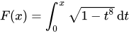




![{\displaystyle f:[-1,1]\to \mathbb {R} ,\ f(t)={\sqrt {1-t^{8}}}}](https://wikimedia.org/api/rest_v1/media/math/render/svg/7e0ab299ac4b6ee8cc92c192b7ec85d263700454)




![{\displaystyle [0,0.5]}](https://wikimedia.org/api/rest_v1/media/math/render/svg/6df34e1c71465ef433a4b08b528287f0276f5282)
![{\displaystyle F(0,5)=\int _{0}^{0.5}{\sqrt {1-t^{8}}}\mathrm {d} t\geq \int _{0}^{0.5}{\sqrt {1-(0.5)^{8}}}\mathrm {d} t=[0.998t]_{0}^{0.5}=0.499\geq 0.496}](https://wikimedia.org/api/rest_v1/media/math/render/svg/20af383932ef9ab4116b57a680338a0f4fc4de56)
![{\displaystyle F(0,5)=\int _{0}^{0.5}{\sqrt {1-t^{8}}}\mathrm {d} t\leq \int _{0}^{0.5}{\sqrt {1-0^{8}}}\mathrm {d} t=[t]_{0}^{0.5}=0.500}](https://wikimedia.org/api/rest_v1/media/math/render/svg/5efc6f2e2c8ef2ef8eb9c93f3c6f6b0818367398)
![{\displaystyle [0,1]}](https://wikimedia.org/api/rest_v1/media/math/render/svg/738f7d23bb2d9642bab520020873cccbef49768d)
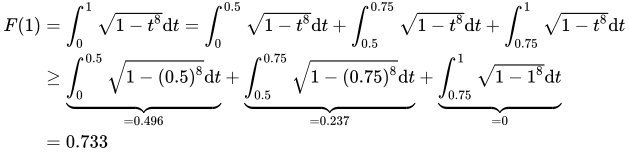



![{\displaystyle ]1,\infty [}](https://wikimedia.org/api/rest_v1/media/math/render/svg/72b3bf6467fe04b9074d5c99b73a8edd26f402f1)






![{\displaystyle ]2,\infty [}](https://wikimedia.org/api/rest_v1/media/math/render/svg/9e735c96946b0ecc3709962b68e70201abb83cd9)
![{\displaystyle ]1,2[}](https://wikimedia.org/api/rest_v1/media/math/render/svg/2f6c3603120c02705bfcc2000141d3497645a429)



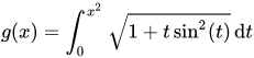


![{\displaystyle [0,x^{2}]}](https://wikimedia.org/api/rest_v1/media/math/render/svg/9006736a45eb18a5d378a9e27a761725bf0d5790)
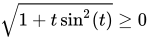

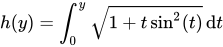

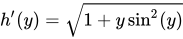
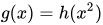



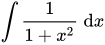


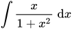
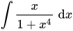
![{\displaystyle {\begin{aligned}&\int {\frac {1}{1+x}}\,\mathrm {d} x\\[0.5em]&{\color {OliveGreen}\left\downarrow \ {\text{Substitution }}y=1+x\Longrightarrow {\frac {\mathrm {d} y}{\mathrm {d} x}}=1\Longrightarrow \mathrm {d} x=\mathrm {d} y\right.}\\[0.5em]&{}=\int {\frac {1}{y}}\,\mathrm {d} y\\[0.5em]&{\color {OliveGreen}\left\downarrow \ {\text{Hauptsatz der Differential- und Integralrechnung}}\right.}\\[0.5em]&{}=\ln(y)+c\\[0.5em]&{\color {OliveGreen}\left\downarrow \ {\text{Rücksubstitution: }}y=1+x\right.}\\[0.5em]&{}=\ln(1+x)+c\end{aligned}}}](https://wikimedia.org/api/rest_v1/media/math/render/svg/2422f8ed45e40ad1f687da9bf5bcffa7b5c6753f)
![{\displaystyle {\begin{aligned}&\int {\frac {1}{1+x^{2}}}\,\mathrm {d} x\\[0.5em]&{\color {OliveGreen}\left\downarrow \ {\text{Hauptsatz der Differential- und Integralrechnung}}\right.}\\[0.5em]&{}=\arctan(x)+c\end{aligned}}}](https://wikimedia.org/api/rest_v1/media/math/render/svg/0239dd758566c288235f1ee63ecb3374bf94a5da)
![{\displaystyle {\begin{aligned}&\int {\frac {x}{1+x}}\,\mathrm {d} x\\[0.5em]&{}=\int {\frac {1+x-1}{1+x}}\,\mathrm {d} x\\[0.5em]&{}=\int \left({\frac {1+x}{1+x}}-{\frac {1}{1+x}}\right)\,\mathrm {d} x\\[0.5em]&{\color {OliveGreen}\left\downarrow \ {\text{Linearität}}\right.}\\[0.5em]&{}=\int 1\,\mathrm {d} x-\int {\frac {1}{1+x}}\,\mathrm {d} x\\[0.5em]&{\color {OliveGreen}\left\downarrow \ {\text{Hauptsatz der Differential- und Integralrechnung und Teilaufgabe 1}}\right.}\\[0.5em]&{}=x-\ln(1+x)+c\end{aligned}}}](https://wikimedia.org/api/rest_v1/media/math/render/svg/d2639df8401f9e77d0d8a42164ad1a1bda0bcbdf)
![{\displaystyle {\begin{aligned}&\int {\frac {x^{2}}{1+x^{2}}}\,\mathrm {d} x\\[0.5em]&{}=\int {\frac {1+x^{2}-1}{1+x^{2}}}\,\mathrm {d} x\\[0.5em]&{}=\int \left({\frac {1+x^{2}}{1+x^{2}}}-{\frac {1}{1+x^{2}}}\right)\,\mathrm {d} x\\[0.5em]&{\color {OliveGreen}\left\downarrow \ {\text{Linearität}}\right.}\\[0.5em]&{}=\int 1\,\mathrm {d} x-\int {\frac {1}{1+x^{2}}}\,\mathrm {d} x\\[0.5em]&{\color {OliveGreen}\left\downarrow \ {\text{Hauptsatz der Differential- und Integralrechnung und Teilaufgabe 2}}\right.}\\[0.5em]&{}=x-\arctan(x)+c\end{aligned}}}](https://wikimedia.org/api/rest_v1/media/math/render/svg/3c445ac61b550f879afac5104003d6a2dfef0e3f)
![{\displaystyle {\begin{aligned}&\int {\frac {x}{1+x^{2}}}\,\mathrm {d} x\\[0.5em]&{\color {OliveGreen}\left\downarrow \ {\text{Substitution }}y=1+x^{2}\Longrightarrow {\frac {\mathrm {d} y}{\mathrm {d} x}}=2x\Longrightarrow \mathrm {d} x={\frac {1}{2x}}\mathrm {d} y\right.}\\[0.5em]&{}=\int {\frac {x}{y}}{\frac {1}{2x}}\,\mathrm {d} y\\[0.5em]&{}=\int {\frac {1}{2}}{\frac {1}{y}}\,\mathrm {d} y\\[0.5em]&{\color {OliveGreen}\left\downarrow \ {\text{Hauptsatz der Differential- und Integralrechnung}}\right.}\\[0.5em]&{}={\frac {1}{2}}\ln(y)+c\\[0.5em]&{\color {OliveGreen}\left\downarrow \ {\text{Rücksubstitution: }}y=1+x^{2}\right.}\\[0.5em]&{}={\frac {1}{2}}\ln(1+x^{2})+c\end{aligned}}}](https://wikimedia.org/api/rest_v1/media/math/render/svg/4128cce58391525b3e092552a535202deda36480)
![{\displaystyle {\begin{aligned}&\int {\frac {x}{1+x^{4}}}\,\mathrm {d} x\\[0.5em]&\int {\frac {x}{1+(x^{2})^{2}}}\,\mathrm {d} x\\[0.5em]&{\color {OliveGreen}\left\downarrow \ {\text{Substitution }}y=x^{2}\Longrightarrow {\frac {\mathrm {d} y}{\mathrm {d} x}}=2x\Longrightarrow \mathrm {d} x={\frac {1}{2x}}\mathrm {d} y\right.}\\[0.5em]&{}=\int {\frac {x}{1+y^{2}}}{\frac {1}{2x}}\,\mathrm {d} y\\[0.5em]&{}=\int {\frac {1}{2}}{\frac {1}{1+y^{2}}}\,\mathrm {d} y\\[0.5em]&{\color {OliveGreen}\left\downarrow \ {\text{Hauptsatz der Differential- und Integralrechnung}}\right.}\\[0.5em]&{}={\frac {1}{2}}\arctan(y)+c\\[0.5em]&{\color {OliveGreen}\left\downarrow \ {\text{Rücksubstitution: }}y=x^{2}\right.}\\[0.5em]&{}={\frac {1}{2}}\arctan(x^{2})+c\end{aligned}}}](https://wikimedia.org/api/rest_v1/media/math/render/svg/3090a603c5c4dd81b4cbf967f486e52729e7b54e)
![{\displaystyle \int {\frac {1}{{\sqrt[{3}]{1-x}}^{4}}}\;\mathrm {d} x}](https://wikimedia.org/api/rest_v1/media/math/render/svg/1bbfb041242e6883fc6222681937de97cc90485f)

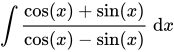
![{\displaystyle x\in ]-{\tfrac {3\pi }{4}},{\tfrac {\pi }{4}}[}](https://wikimedia.org/api/rest_v1/media/math/render/svg/f0f0f9d4779e9ffa6320d24a877f78dd5de89b5a)
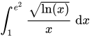
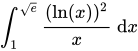
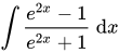
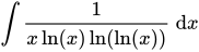

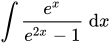

![{\displaystyle \int _{1}^{e}{\frac {\ln(x)}{x([\ln(x)]^{2}+1)}}\;\mathrm {d} x}](https://wikimedia.org/api/rest_v1/media/math/render/svg/ac0395354bad1e5cce61d6cc425f5ec36457ab08)
![{\displaystyle {\begin{aligned}&\int {\frac {1}{{\sqrt[{3}]{1-x}}^{4}}}\,\mathrm {d} x\\[0.5em]&\int {\frac {1}{(1-x)^{\frac {4}{3}}}}\,\mathrm {d} x\\[0.5em]&{\color {OliveGreen}\left\downarrow \ {\text{Substitution }}y=1-x\Longrightarrow {\frac {\mathrm {d} y}{\mathrm {d} x}}=-1\Longrightarrow \mathrm {d} x=-\mathrm {d} y\right.}\\[0.5em]&=-\int {\frac {1}{y^{\frac {4}{3}}}}\,\mathrm {d} y\\[0.5em]&=-\int y^{-{\frac {4}{3}}}\,\mathrm {d} y\\[0.5em]&{\color {OliveGreen}\left\downarrow \ {\text{Hauptsatz der Differential- und Integralrechnung}}\right.}\\[0.5em]&=-(-3y^{-{\frac {1}{3}}})+c\\[0.5em]&=3y^{-{\frac {1}{3}}}+c\\[0.5em]&{\color {OliveGreen}\left\downarrow \ {\text{Rücksubstitution: }}y=1+x\right.}\\[0.5em]&=3(1-x)^{-{\frac {1}{3}}}+c\end{aligned}}}](https://wikimedia.org/api/rest_v1/media/math/render/svg/5b0da20d6b68da47badd1ab51921dc2b12818158)
![{\displaystyle {\begin{aligned}&\int {\frac {\cos(x)+\sin(x)}{\cos(x)-\sin(x)}}\,\mathrm {d} x\\[0.5em]&=-\int {\frac {\cos(x)+\sin(x)}{\sin(x)-\cos(x)}}\,\mathrm {d} x\\[0.5em]&{\color {OliveGreen}\left\downarrow \ {\text{Substitution }}y=\sin(x)-\cos(x)\Longrightarrow {\frac {\mathrm {d} y}{\mathrm {d} x}}=\cos(x)+\sin(x)\Longrightarrow \mathrm {d} x={\frac {1}{\cos(x)+\sin(x)}}\mathrm {d} y\right.}\\[0.5em]&=-\int {\frac {1}{y}}\,\mathrm {d} y\\[0.5em]&{\color {OliveGreen}\left\downarrow \ {\text{Hauptsatz der Differential- und Integralrechnung}}\right.}\\[0.5em]&=-\ln |y|+c\\[0.5em]&{\color {OliveGreen}\left\downarrow \ {\text{Rücksubstitution: }}y=\sin(x)-\cos(x)\right.}\\[0.5em]&=-\ln |\sin(x)-\cos(x)|+c\end{aligned}}}](https://wikimedia.org/api/rest_v1/media/math/render/svg/d969522a915867aa945186f448f069f91ce87c50)
![{\displaystyle {\begin{aligned}&\int _{1}^{e^{2}}{\frac {\sqrt {\ln(x)}}{x}}\;\mathrm {d} x\\[0.5em]&{\color {OliveGreen}\left\downarrow \ {\text{Substitution }}y=\ln(x)\Longrightarrow {\frac {\mathrm {d} y}{\mathrm {d} x}}={\frac {1}{x}}\Longrightarrow \mathrm {d} x=x\mathrm {d} y\right.}\\[0.5em]&=\int _{\ln(1)}^{\ln(e^{2})}{\sqrt {y}}\,\mathrm {d} y\\[0.5em]&=\int _{0}^{2}y^{\frac {1}{2}}\,\mathrm {d} y\\[0.5em]&{\color {OliveGreen}\left\downarrow \ {\text{Hauptsatz der Differential- und Integralrechnung}}\right.}\\[0.5em]&=\left[{\frac {2}{3}}y^{\frac {3}{2}}\right]_{0}^{2}\\[0.5em]&={\frac {2}{3}}\cdot 2^{\frac {3}{2}}-{\frac {2}{3}}\cdot 0\\[0.5em]&={\frac {2}{3}}\cdot 2{\sqrt {2}}\\[0.5em]&={\frac {4{\sqrt {2}}}{3}}\end{aligned}}}](https://wikimedia.org/api/rest_v1/media/math/render/svg/d17f616cc1f0e9189d94ad465f3346057852c5fe)
![{\displaystyle {\begin{aligned}&\int _{1}^{\sqrt {e}}{\frac {(\ln(x))^{2}}{x}}\;\mathrm {d} x\\[0.5em]&{\color {OliveGreen}\left\downarrow \ {\text{Substitution }}y=\ln(x)\Longrightarrow {\frac {\mathrm {d} y}{\mathrm {d} x}}={\frac {1}{x}}\Longrightarrow \mathrm {d} x=x\mathrm {d} y\right.}\\[0.5em]&=\int _{\ln(1)}^{\ln({\sqrt {e}})}y^{2}\,\mathrm {d} y\\[0.5em]&=\int _{0}^{\frac {1}{2}}y^{2}\,\mathrm {d} y\\[0.5em]&{\color {OliveGreen}\left\downarrow \ {\text{Hauptsatz der Differential- und Integralrechnung}}\right.}\\[0.5em]&=\left[{\frac {1}{3}}y^{3}\right]_{0}^{\frac {1}{2}}\\[0.5em]&={\frac {1}{3}}\cdot \left({\frac {1}{2}}\right)^{3}-{\frac {1}{3}}\cdot 0\\[0.5em]&={\frac {1}{3}}\cdot {\frac {1}{8}}\\[0.5em]&={\frac {1}{24}}\end{aligned}}}](https://wikimedia.org/api/rest_v1/media/math/render/svg/c58137ca620214d3dffc7d8a0eaa37873ce1c4ce)
![{\displaystyle {\begin{aligned}&\int {\frac {e^{2x}-1}{e^{2x}+1}}\;\mathrm {d} x\\[0.5em]&\ =\int {\frac {e^{x}(e^{x}-e^{-x})}{e^{x}(e^{x}+e^{-x})}}\;\mathrm {d} x\\[0.5em]&\ =\int {\frac {e^{x}-e^{-x}}{e^{x}+e^{-x}}}\;\mathrm {d} x\\[0.5em]&{\color {OliveGreen}\left\downarrow \ {\text{Substitution }}y=e^{x}+e^{-x}\Longrightarrow {\frac {\mathrm {d} y}{\mathrm {d} x}}=e^{x}-e^{-x}\Longrightarrow \mathrm {d} x={\frac {1}{e^{x}-e^{-x}}}\mathrm {d} y\right.}\\[0.5em]&\ =\int {\frac {1}{y}}\,\mathrm {d} y\\[0.5em]&{\color {OliveGreen}\left\downarrow \ {\text{Hauptsatz der Differential- und Integralrechnung}}\right.}\\[0.5em]&\ =\ln(y)+c\\[0.5em]&{\color {OliveGreen}\left\downarrow \ {\text{Rücksubstitution: }}y=e^{x}+e^{-x}\right.}\\[0.5em]&\ =\ln(e^{x}+e^{-x})+c\end{aligned}}}](https://wikimedia.org/api/rest_v1/media/math/render/svg/ef781ca909db02393dffe613fcdf7d6e4c1df477)
![{\displaystyle {\begin{aligned}&\int {\frac {e^{2x}-1}{e^{2x}+1}}\;\mathrm {d} x\\[0.5em]&\ =\int {\frac {e^{x}(e^{x}-e^{-x})}{e^{x}(e^{x}+e^{-x})}}\;\mathrm {d} x\\[0.5em]&\ =\int {\frac {e^{x}-e^{-x}}{e^{x}+e^{-x}}}\;\mathrm {d} x\\[0.5em]&\ =\int {\frac {\sinh(x)}{\cosh(x)}}\;\mathrm {d} x\\[0.5em]&{\color {OliveGreen}\left\downarrow \ {\text{Substitution }}y=\cosh(x)\Longrightarrow {\frac {\mathrm {d} y}{\mathrm {d} x}}=\sinh(x)\Longrightarrow \mathrm {d} x={\frac {1}{\sinh(x)}}\mathrm {d} y\right.}\\[0.5em]&\ =\int {\frac {1}{y}}\,\mathrm {d} y\\[0.5em]&{\color {OliveGreen}\left\downarrow \ {\text{Hauptsatz der Differential- und Integralrechnung}}\right.}\\[0.5em]&\ =\ln(y)+c\\[0.5em]&{\color {OliveGreen}\left\downarrow \ {\text{Rücksubstitution: }}y=\cosh(x)\right.}\\[0.5em]&\ =\ln(\cosh(x))+c\end{aligned}}}](https://wikimedia.org/api/rest_v1/media/math/render/svg/d3cd35d2ddbdc32cbd094ba059be30d6de8e9a98)
![{\displaystyle {\begin{aligned}&\int {\frac {e^{2x}-1}{e^{2x}+1}}\;\mathrm {d} x\\[0.5em]&\ =\int {\frac {2e^{2x}-1-e^{2x}}{e^{2x}+1}}\;\mathrm {d} x\\[0.5em]&\ =\int {\frac {2e^{2x}-(e^{2x}+1)}{e^{2x}+1}}\;\mathrm {d} x\\[0.5em]&\ =\int \left({\frac {2e^{2x}}{e^{2x}+1}}-{\frac {e^{2x}+1}{e^{2x}+1}}\right)\;\mathrm {d} x\\[0.5em]&{\color {OliveGreen}\left\downarrow \ {\text{Linearität des Integrals}}\right.}\\[0.5em]&\ =\int {\frac {2e^{2x}}{e^{2x}+1}}\;\mathrm {d} x-\int \underbrace {\frac {e^{2x}+1}{e^{2x}+1}} _{=1}\;\mathrm {d} x\\[0.5em]&{\color {OliveGreen}\left\downarrow \ {\text{Substitution }}y=e^{2x}+1\Longrightarrow {\frac {\mathrm {d} y}{\mathrm {d} x}}=2e^{2x}\Longrightarrow \mathrm {d} x={\frac {1}{2e^{2x}}}\mathrm {d} y\right.}\\[0.5em]&\ =\int {\frac {1}{y}}\,\mathrm {d} y-\int 1\,\mathrm {d} x\\[0.5em]&{\color {OliveGreen}\left\downarrow \ {\text{Hauptsatz der Differential- und Integralrechnung}}\right.}\\[0.5em]&\ =\ln(y)-x+c\\[0.5em]&{\color {OliveGreen}\left\downarrow \ {\text{Rücksubstitution: }}y=e^{2x}+1\right.}\\[0.5em]&\ =\ln(e^{2x}+1)-x+c\end{aligned}}}](https://wikimedia.org/api/rest_v1/media/math/render/svg/6b7b313de246a6e055120d71cf69b8c398422be0)
![{\displaystyle {\begin{aligned}&\int {\frac {1}{x\ln(x)\ln(\ln(x))}}\;\mathrm {d} x\\[0.5em]&{\color {OliveGreen}\left\downarrow \ {\text{Substitution }}y=\ln(\ln(x))\Longrightarrow {\frac {\mathrm {d} y}{\mathrm {d} x}}={\frac {1}{x\ln(x)}}\Longrightarrow \mathrm {d} x=x\ln(x)\mathrm {d} y\right.}\\[0.5em]&\ =\int {\frac {1}{y}}\;\mathrm {d} y\\[0.5em]&{\color {OliveGreen}\left\downarrow \ {\text{Hauptsatz der Differential- und Integralrechnung}}\right.}\\[0.5em]&\ =\ln(y)+c\\[0.5em]&{\color {OliveGreen}\left\downarrow \ {\text{Rücksubstitution: }}y=\ln(\ln(x))\right.}\\[0.5em]&\ =\ln(\ln(\ln(x)))+c\end{aligned}}}](https://wikimedia.org/api/rest_v1/media/math/render/svg/e9d852bd79cef5de1c432b693e7fa9c133715766)
![{\displaystyle {\begin{aligned}&\int {\frac {e^{x}}{e^{2x}-1}}\;\mathrm {d} x\\[0.5em]&\ =\int {\frac {e^{x}}{(e^{x})^{2}-1}}\;\mathrm {d} x\\[0.5em]&{\color {OliveGreen}\left\downarrow \ {\text{Substitution }}y=e^{x}\Longrightarrow {\frac {\mathrm {d} y}{\mathrm {d} x}}=e^{x}\Longrightarrow \mathrm {d} x={\frac {1}{e^{x}}}\mathrm {d} y\ (x<0\Longrightarrow y\in (0,1))\right.}\\[0.5em]&\ =\int {\frac {1}{y^{2}-1}}\;\mathrm {d} y\\[0.5em]&\ =-\int {\frac {1}{1-y^{2}}}\;\mathrm {d} y\\[0.5em]&{\color {OliveGreen}\left\downarrow \ {\text{Hauptsatz der Differential- und Integralrechnung}}\right.}\\[0.5em]&\ =-{\text{artanh}}(y)+c\\[0.5em]&{\color {OliveGreen}\left\downarrow \ {\text{Rücksubstitution: }}y=e^{x}\right.}\\[0.5em]&\ =-{\text{artanh}}(e^{x})+c\end{aligned}}}](https://wikimedia.org/api/rest_v1/media/math/render/svg/89c7b91dc28ed4a4c917fed97e7bf24fc6a12a9d)
![{\displaystyle {\begin{aligned}&\int _{1}^{e}{\frac {\ln(x)}{x([\ln(x)]^{2}+1)}}\;\mathrm {d} x\\[0.5em]&{\color {OliveGreen}\left\downarrow \ {\text{Substitution }}y=\ln(x)\Longrightarrow {\frac {\mathrm {d} y}{\mathrm {d} x}}={\frac {1}{x}}\Longrightarrow \mathrm {d} x=x\mathrm {d} y\right.}\\[0.5em]&\ =\int _{\ln(1)}^{\ln(e)}{\frac {y}{y^{2}+1}}\;\mathrm {d} y\\[0.5em]&\ =\int _{0}^{1}{\frac {y}{y^{2}+1}}\;\mathrm {d} y\\[0.5em]&{\color {OliveGreen}\left\downarrow \ {\text{Substitution }}t=y^{2}+1\Longrightarrow {\frac {\mathrm {d} t}{\mathrm {d} y}}=2y\Longrightarrow \mathrm {d} y={\frac {1}{2y}}\mathrm {d} t\right.}\\[0.5em]&\ =\int _{0^{2}+1}^{1^{2}+1}{\frac {1}{2t}}\;\mathrm {d} t\\[0.5em]&\ ={\frac {1}{2}}\int _{1}^{2}{\frac {1}{t}}\;\mathrm {d} t\\[0.5em]&{\color {OliveGreen}\left\downarrow \ {\text{Hauptsatz der Differential- und Integralrechnung}}\right.}\\[0.5em]&\ ={\frac {1}{2}}\left[\ln(t)\right]_{1}^{2}\\[0.5em]&\ ={\frac {1}{2}}[\ln(2)-\ln(1)]\\[0.5em]&\ ={\frac {1}{2}}\ln(2)\end{aligned}}}](https://wikimedia.org/api/rest_v1/media/math/render/svg/0a75d8377cf62d27cfe80f4794adeadef0dd693f)
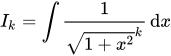

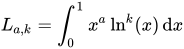


![{\displaystyle {\begin{aligned}I_{k}&=\int {\frac {1}{{\sqrt {1+x^{2}}}^{k}}}\,\mathrm {d} x\\[0.5em]&=\int 1\cdot {\frac {1}{(1+x^{2})^{\tfrac {k}{2}}}}\,\mathrm {d} x\\[0.5em]&{\color {OliveGreen}\left\downarrow \ {\text{Partielle Integration mit}}\ f'(x)=1\ {\text{und}}\ g(x)={\frac {1}{(1+x^{2})^{\tfrac {k}{2}}}}\Longrightarrow f(x)=x\ {\text{und}}\ g'(x)=-{\frac {k}{2}}{\frac {1}{(1+x^{2})^{{\tfrac {k}{2}}+1}}}\cdot 2x=-k{\frac {x}{(1+x^{2})^{{\tfrac {k}{2}}+1}}}\right.}\\[0.5em]&{}=x\cdot {\frac {1}{{\sqrt {1+x^{2}}}^{k}}}-\int x\cdot \left(-k{\frac {x}{(1+x^{2})^{{\tfrac {k}{2}}+1}}}\right)\,\mathrm {d} x\\[0.5em]&{}={\frac {x}{{\sqrt {1+x^{2}}}^{k}}}+k\int {\frac {x^{2}}{(1+x^{2})^{{\tfrac {k}{2}}+1}}}\,\mathrm {d} x\\[0.5em]&{}={\frac {x}{{\sqrt {1+x^{2}}}^{k}}}+k\int {\frac {1+x^{2}-1}{(1+x^{2})^{{\tfrac {k}{2}}+1}}}\,\mathrm {d} x\\[0.5em]&{}={\frac {x}{{\sqrt {1+x^{2}}}^{k}}}+k\int \left({\frac {1+x^{2}}{(1+x^{2})^{{\tfrac {k}{2}}+1}}}-{\frac {1}{(1+x^{2})^{{\tfrac {k}{2}}+1}}}\right)\,\mathrm {d} x\\[0.5em]&{}={\frac {x}{{\sqrt {1+x^{2}}}^{k}}}+\underbrace {k\int {\frac {1}{(1+x^{2})^{\tfrac {k}{2}}}}\,\mathrm {d} x} _{=k\cdot I_{k}}-\underbrace {k\int {\frac {1}{(1+x^{2})^{\tfrac {k+2}{2}}}}} _{=k\cdot I_{k+2}}\,\mathrm {d} x\end{aligned}}}](https://wikimedia.org/api/rest_v1/media/math/render/svg/b251e1a6e986876a1c7cd7e19cc6da9af24ad64e)
![{\displaystyle {\begin{aligned}&k\cdot I_{k+2}=(k-1)\cdot I_{k}+{\frac {x}{{\sqrt {1+x^{2}}}^{k}}}\\[0.5cm]{\overset {|:k}{\iff }}&I_{k+2}={\frac {k-1}{k}}\cdot I_{k}+{\frac {x}{k{\sqrt {1+x^{2}}}^{k}}}\end{aligned}}}](https://wikimedia.org/api/rest_v1/media/math/render/svg/91cadd7d956975fadf8bc0c2a37d37c50bad0d53)





![{\displaystyle {\begin{aligned}I_{1}&=\int {\frac {1}{\sqrt {1+x^{2}}}}\,\mathrm {d} x\\[0.5cm]&=\int {\frac {1}{\sqrt {1+x^{2}}}}\cdot {\frac {x+{\sqrt {1+x^{2}}}}{x+{\sqrt {1+x^{2}}}}}\,\mathrm {d} x\\[0.5cm]&=\int {\frac {{\frac {1}{\sqrt {1+x^{2}}}}\cdot (x+{\sqrt {1+x^{2}}})}{x+{\sqrt {1+x^{2}}}}}\,\mathrm {d} x\\[0.5cm]&=\int {\frac {{\frac {x}{\sqrt {1+x^{2}}}}+1}{x+{\sqrt {1+x^{2}}}}}\,\mathrm {d} x\\[0.5cm]&=\ln(x+{\sqrt {1+x^{2}}})\end{aligned}}}](https://wikimedia.org/api/rest_v1/media/math/render/svg/2e9f954bd17386876f90ea17e1f75918754bb312)

![{\displaystyle {\begin{aligned}L_{a,k}&=\int _{0}^{1}x^{a}\ln ^{k}(x)\,\mathrm {d} x\\[0.5em]&{\color {OliveGreen}\left\downarrow \ {\text{Partielle Integration mit}}\ f'(x)=x^{a}\ {\text{und}}\ g(x)=\ln ^{k}(x)\Longrightarrow f(x)={\frac {1}{a+1}}x^{a+1}\ {\text{und}}\ g'(x)=k\ln ^{k-1}(x)\cdot {\frac {1}{x}}={\frac {k\ln ^{k-1}(x)}{x}}\right.}\\[0.5em]&{}=\underbrace {\left[{\frac {x^{a+1}\ln ^{k}(x)}{a+1}}\right]_{0}^{1}} _{=0}-\int _{0}^{1}{\frac {k}{a+1}}{\frac {x^{a+1}\ln ^{k-1}(x)}{x}}\,\mathrm {d} x\\[0.5em]&{}=\left[\underbrace {\frac {1^{a+1}\ln ^{k}(1)}{a+1}} _{=0}-\underbrace {\lim _{x\to 0+}{\frac {x^{a+1}\ln ^{k}(x)}{a+1}}} _{=0}\right]-\int _{0}^{1}{\frac {k}{a+1}}{\frac {x^{a+1}\ln ^{k-1}(x)}{x}}\,\mathrm {d} x\\[0.5em]&{}=-{\frac {k}{a+1}}\int _{0}^{1}x^{a}\ln ^{k-1}(x)\,\mathrm {d} x\\[0.5em]&{}=-{\frac {k}{a+1}}L_{a,k-1}\end{aligned}}}](https://wikimedia.org/api/rest_v1/media/math/render/svg/cd1be86fab8a00fc1a5407a3ec13dfff0b08df8c)

![{\displaystyle {\begin{aligned}L_{a,k}&=(-1)^{k}{\frac {k!}{(a+1)^{k}}}L_{a,0}\\[0.5cm]&=(-1)^{k}{\frac {k!}{(a+1)^{k}}}\int _{0}^{1}x^{a}\ln ^{0}(x)\,\mathrm {d} x\\[0.5cm]&=(-1)^{k}{\frac {k!}{(a+1)^{k}}}\int _{0}^{1}x^{a}\,\mathrm {d} x\\[0.5cm]&=(-1)^{k}{\frac {k!}{(a+1)^{k}}}\left[{\frac {x^{a+1}}{a+1}}\right]_{0}^{1}\\[0.5cm]&=(-1)^{k}{\frac {k!}{(a+1)^{k}}}{\frac {1}{a+1}}\\[0.5cm]&=(-1)^{k}{\frac {k!}{(a+1)^{k+1}}}\end{aligned}}}](https://wikimedia.org/api/rest_v1/media/math/render/svg/7c59d70e39d43bbec862ddc5d2bbcf9146569033)

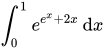
![{\displaystyle {\begin{aligned}&\int e^{e^{x}+x}\,\mathrm {d} x\\[0.3em]=\ &\int e^{e^{x}}\cdot e^{x}\,\mathrm {d} x\\[0.3em]&{\color {OliveGreen}\left\downarrow \ {\text{Substitution:}}\ y=e^{x}\Longrightarrow {\frac {\mathrm {d} y}{\mathrm {d} x}}=e^{x}\Longrightarrow \mathrm {d} x={\frac {1}{e^{x}}}\mathrm {d} y\right.}\\[0.3em]=\ &\int e^{y}\,\mathrm {d} y\\[0.3em]&{\color {OliveGreen}\left\downarrow \ {\text{Hauptsatz der Differential- und Integralrechnung mit}}\ f(y)=e^{y}\Longrightarrow F(y)=e^{y}+c\right.}\\[0.3em]=\ &e^{y}+c\\[0.3em]&{\color {OliveGreen}\left\downarrow \ {\text{Rücksubstitution:}}\ y=e^{x}\right.}\\[0.3em]=\ &e^{e^{x}}+c\end{aligned}}}](https://wikimedia.org/api/rest_v1/media/math/render/svg/8df4c8585b1267a9994925194b9478b1fad3de8e)


![{\displaystyle {\begin{aligned}&\int _{0}^{1}e^{e^{x}+2x}\,\mathrm {d} x\\[0.3em]=\ &\int _{0}^{1}e^{e^{x}+x}\cdot e^{x}\,\mathrm {d} x\\[0.3em]&{\color {OliveGreen}\left\downarrow \ {\text{Partielle Integration mit}}\ f'(x)=e^{e^{x}+x}\ {\text{und}}\ g(x)=e^{x}\Longrightarrow f(x)=e^{e^{x}}\ {\text{und}}\ g'(x)=e^{x}\right.}\\[0.3em]=\ &[e^{e^{x}}\cdot e^{x}]_{0}^{1}-\int _{0}^{1}e^{e^{x}}\cdot e^{x}\,\mathrm {d} x\\[0.3em]&{\color {OliveGreen}\left\downarrow \ {\text{Hauptsatz der Differential- und Integralrechnung mit}}\ f(x)=e^{e^{x}}\cdot e^{x}\Longrightarrow F(x)=e^{e^{x}}\right.}\\[0.3em]=\ &e^{e}\cdot e-e-[e^{e^{x}}]_{0}^{1}\\[0.3em]=\ &e^{e}\cdot e-e-e^{e}+e\\[0.3em]=\ &e^{e}\cdot (e-1)\end{aligned}}}](https://wikimedia.org/api/rest_v1/media/math/render/svg/6baf443c169aaeec98c587b89839a37c5694301e)

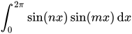
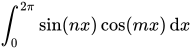


![{\displaystyle {\begin{aligned}&\int _{0}^{2\pi }\sin(nx)\sin(nx)\,\mathrm {d} x\\[0.3em]&=\int _{0}^{2\pi }\sin ^{2}(nx)\,\mathrm {d} x\\[0.3cm]&{\color {OliveGreen}\left\downarrow \ {\text{Substitution:}}\ y=nx\Longrightarrow {\frac {\mathrm {d} y}{\mathrm {d} x}}=n\Longrightarrow \mathrm {d} x={\frac {1}{n}}\mathrm {d} y\right.}\\[0.3em]&={\frac {1}{n}}\int _{0}^{2\pi n}\sin ^{2}(y)\,\mathrm {d} y\\[0.3cm]&{\color {OliveGreen}\left\downarrow \ \int \sin ^{2}(x)\,\mathrm {d} x=-{\frac {1}{2}}\cos(x)\sin(x)+{\frac {1}{2}}x\right.}\\[0.3em]&={\frac {1}{n}}\left[-{\frac {1}{2}}\cos(x)\sin(x)+{\frac {1}{2}}x\right]_{0}^{2\pi n}\\[0.3ex]&={\frac {1}{n}}\left[\underbrace {-{\frac {1}{2}}\cos(2\pi n)\sin(2\pi n)} _{=0}+{\frac {1}{2}}\cdot 2\pi n-\underbrace {(-{\frac {1}{2}}\cos(0)\sin(0)+{\frac {1}{2}}\cdot 0} _{=0}\right]\\[0.3em]&={\frac {1}{n}}\cdot {\frac {1}{2}}\cdot 2\pi n\\[0.3em]&=\pi \end{aligned}}}](https://wikimedia.org/api/rest_v1/media/math/render/svg/e0321f8b52a9d36c4391cc384b25d4cfa9f0992b)
![{\displaystyle {\begin{aligned}&\int _{0}^{2\pi }\sin(nx)\sin(mx)\,\mathrm {d} x\\[0.3cm]&{\color {OliveGreen}\left\downarrow \ {\text{Partielle Integration mit}}\ f'(x)=\sin(nx)\ {\text{und}}\ g(x)=\sin(mx)\Longrightarrow f(x)=-{\frac {1}{n}}\cos(nx)\ {\text{und}}\ g'(x)=m\cos(mx)\right.}\\[0.3em]&=\underbrace {\left[-{\frac {1}{n}}\cos(nx)\sin(mx)\right]_{0}^{2\pi }} _{=0}-\int _{0}^{2\pi }\left(-{\frac {m}{n}}\cos(nx)\cos(mx)\right)\,\mathrm {d} x\\[0.3em]&={\frac {m}{n}}\int _{0}^{2\pi }\cos(nx)\cos(mx)\,\mathrm {d} x\\[0.3em]&{\color {OliveGreen}\left\downarrow \ {\text{Partielle Integration mit}}\ f'(x)=\cos(nx)\ {\text{und}}\ g(x)=\cos(mx)\Longrightarrow f(x)={\frac {1}{n}}\sin(nx)\ {\text{und}}\ g'(x)=-m\sin(mx)\right.}\\[0.3em]&={\frac {m}{n}}\cdot \underbrace {\left[{\frac {1}{n}}\sin(nx)\cos(mx)\right]_{0}^{2\pi }} _{=0}-{\frac {m}{n}}\int _{0}^{2\pi }\left(-{\frac {m}{n}}\sin(nx)\sin(mx)\right)\,\mathrm {d} x\\[0.3em]&={\frac {m^{2}}{n^{2}}}\int _{0}^{2\pi }\sin(nx)\sin(mx)\,\mathrm {d} x\end{aligned}}}](https://wikimedia.org/api/rest_v1/media/math/render/svg/644bdeed880ae4aacdac1d2dbd4a4519b6ccad3d)
![{\displaystyle {\begin{aligned}&\int _{0}^{2\pi }\sin(nx)\sin(mx)\,\mathrm {d} x-{\frac {m^{2}}{n^{2}}}\int _{0}^{2\pi }\sin(nx)\sin(mx)\,\mathrm {d} x=0\\[0.3em]\iff &\underbrace {\left(1-{\frac {m^{2}}{n^{2}}}\right)} _{\neq 0}\int _{0}^{2\pi }\sin(nx)\sin(mx)\,\mathrm {d} x=0\end{aligned}}}](https://wikimedia.org/api/rest_v1/media/math/render/svg/f5faf9475ff8b23969de3b7909692f994ee479a4)
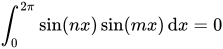
![{\displaystyle {\begin{aligned}&\int _{0}^{2\pi }\sin(nx)\cos(nx)\,\mathrm {d} x\\[0.3cm]&{\color {OliveGreen}\left\downarrow \ {\text{Substitution:}}\ y=nx\Longrightarrow {\frac {\mathrm {d} y}{\mathrm {d} x}}=n\Longrightarrow \mathrm {d} x={\frac {1}{n}}\mathrm {d} y\right.}\\[0.3em]&={\frac {1}{n}}\int _{0}^{2\pi n}\sin(y)\cos(y)\,\mathrm {d} y\\[0.3cm]&{\color {OliveGreen}\left\downarrow \ \int \sin(x)\cos(x)\,\mathrm {d} x=-{\frac {1}{2}}\cos ^{2}(x)\right.}\\[0.3em]&={\frac {1}{n}}\left[-{\frac {1}{2}}\cos ^{2}(x)\right]_{0}^{2\pi n}\\[0.3ex]&={\frac {1}{n}}\left[-{\frac {1}{2}}\cos ^{2}(2\pi n)-(-{\frac {1}{2}}\cos ^{2}(0))\right]\\[0.3em]&={\frac {1}{n}}\left[-{\frac {1}{2}}+{\frac {1}{2}}\right]\\[0.3em]&={\frac {1}{n}}\cdot 0\\[0.3em]&=0\end{aligned}}}](https://wikimedia.org/api/rest_v1/media/math/render/svg/f880caf2c4b05e894495bf016a6942bda52fb6d7)
![{\displaystyle {\begin{aligned}&\int _{0}^{2\pi }\sin(nx)\cos(mx)\,\mathrm {d} x\\[0.3cm]&{\color {OliveGreen}\left\downarrow \ {\text{Partielle Integration mit}}\ f'(x)=\sin(nx)\ {\text{und}}\ g(x)=\cos(mx)\Longrightarrow f(x)=-{\frac {1}{n}}\cos(nx)\ {\text{und}}\ g'(x)=-m\sin(mx)\right.}\\[0.3em]&=\underbrace {\left[-{\frac {1}{n}}\cos(nx)\cos(mx)\right]_{0}^{2\pi }} _{=0}-\int _{0}^{2\pi }\left({\frac {m}{n}}\cos(nx)\sin(mx)\right)\,\mathrm {d} x\\[0.3em]&=-{\frac {m}{n}}\int _{0}^{2\pi }\cos(nx)\sin(mx)\,\mathrm {d} x\\[0.3em]&{\color {OliveGreen}\left\downarrow \ {\text{Partielle Integration mit}}\ f'(x)=\cos(nx)\ {\text{und}}\ g(x)=\sin(mx)\Longrightarrow f(x)={\frac {1}{n}}\sin(nx)\ {\text{und}}\ g'(x)=m\cos(mx)\right.}\\[0.3em]&={\frac {m}{n}}\cdot \underbrace {\left[{\frac {1}{n}}\sin(nx)\sin(mx)\right]_{0}^{2\pi }} _{=0}-\left[-{\frac {m}{n}}\int _{0}^{2\pi }\left({\frac {m}{n}}\sin(nx)\cos(mx)\right)\,\mathrm {d} x\right]\\[0.3em]&={\frac {m^{2}}{n^{2}}}\int _{0}^{2\pi }\sin(nx)\cos(mx)\,\mathrm {d} x\end{aligned}}}](https://wikimedia.org/api/rest_v1/media/math/render/svg/ff9102a19043602fafe6f9cc3056f4d0bf5b242f)

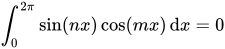
![{\displaystyle {\begin{aligned}&\int _{0}^{2\pi }\cos(nx)\cos(nx)\,\mathrm {d} x\\[0.3em]&=\int _{0}^{2\pi }\cos ^{2}(nx)\,\mathrm {d} x\\[0.3cm]&{\color {OliveGreen}\left\downarrow \ {\text{Substitution:}}\ y=nx\Longrightarrow {\frac {\mathrm {d} y}{\mathrm {d} x}}=n\Longrightarrow \mathrm {d} x={\frac {1}{n}}\mathrm {d} y\right.}\\[0.3em]&={\frac {1}{n}}\int _{0}^{2\pi n}\cos ^{2}(y)\,\mathrm {d} y\\[0.3cm]&{\color {OliveGreen}\left\downarrow \ \int \cos ^{2}(x)\,\mathrm {d} x={\frac {1}{2}}\cos(x)\sin(x)+{\frac {1}{2}}x\right.}\\[0.3em]&={\frac {1}{n}}\left[{\frac {1}{2}}\cos(x)\sin(x)+{\frac {1}{2}}x\right]_{0}^{2\pi n}\\[0.3ex]&={\frac {1}{n}}\left[\underbrace {{\frac {1}{2}}\cos(2\pi n)\sin(2\pi n)} _{=0}+{\frac {1}{2}}\cdot 2\pi n-\underbrace {(-{\frac {1}{2}}\cos(0)\sin(0)+{\frac {1}{2}}\cdot 0} _{=0}\right]\\[0.3em]&={\frac {1}{n}}\cdot {\frac {1}{2}}\cdot 2\pi n\\[0.3em]&=\pi \end{aligned}}}](https://wikimedia.org/api/rest_v1/media/math/render/svg/394eb85663ab3b1b4669732191ebcf5062cfe65b)
![{\displaystyle {\begin{aligned}&\int _{0}^{2\pi }\cos(nx)\cos(mx)\,\mathrm {d} x\\[0.3cm]&{\color {OliveGreen}\left\downarrow \ {\text{Partielle Integration mit}}\ f'(x)=\cos(nx)\ {\text{und}}\ g(x)=\cos(mx)\Longrightarrow f(x)={\frac {1}{n}}\sin(nx)\ {\text{und}}\ g'(x)=-m\sin(mx)\right.}\\[0.3em]&=\underbrace {\left[{\frac {1}{n}}\sin(nx)\cos(mx)\right]_{0}^{2\pi }} _{=0}-\int _{0}^{2\pi }\left(-{\frac {m}{n}}\sin(nx)\sin(mx)\right)\,\mathrm {d} x\\[0.3em]&={\frac {m}{n}}\int _{0}^{2\pi }\sin(nx)\sin(mx)\,\mathrm {d} x\\[0.3em]&{\color {OliveGreen}\left\downarrow \ \int _{0}^{2\pi }\sin(nx)\sin(mx)\,\mathrm {d} x=0\ {\text{nach Teilaufgabe 1}}\ \right.}\\[0.3em]&={\frac {m}{n}}\cdot 0\\[0.3em]&=0\end{aligned}}}](https://wikimedia.org/api/rest_v1/media/math/render/svg/c75c7bae0a9c8f981783d2bb7dfe2c4bd71bfdde)
![{\displaystyle f:[0,1]\to [0,1]}](https://wikimedia.org/api/rest_v1/media/math/render/svg/f64956bbc19d5bbe642fd7bf4f1aa62487006f4d)


![{\displaystyle x\in [0,1]}](https://wikimedia.org/api/rest_v1/media/math/render/svg/64a15936df283add394ab909aa7a5e24e7fb6bb2)

![{\displaystyle {\begin{aligned}&\int _{0}^{1}\!f^{-1}(y)\,\mathrm {d} y\\[0.3em]&{\color {OliveGreen}\left\downarrow \ {\text{Substitution:}}\ y=f(x)\Longrightarrow {\frac {\mathrm {d} y}{\mathrm {d} x}}=f'(x)\Longrightarrow \mathrm {d} y=f'(x)\mathrm {d} x\right.}\\[0.3em]=\ &\int _{f(0)}^{f(1)}f^{-1}(f(x))\cdot f'(x)\,\mathrm {d} x\\[0.3em]&{\color {OliveGreen}\left\downarrow \ f(0)=0,\ f(1)=1\ {\text{und}}\ f^{-1}(f(x))=x\right.}\\[0.3em]=\ &\int _{0}^{1}x\cdot f'(x)\,\mathrm {d} x\\[0.3em]&{\color {OliveGreen}\left\downarrow \ {\text{Partielle Integration mit}}\ f'(x)=f'(x)\ {\text{und}}\ g(x)=x\Longrightarrow f(x)=f(x)\ {\text{und}}\ g'(x)=1\right.}\\[0.3em]=\ &[x\cdot f(x)]_{0}^{1}-\int _{0}^{1}1\cdot f(x)\,\mathrm {d} x\\[0.3em]=\ &1\cdot \underbrace {f(1)} _{=1}-\underbrace {0\cdot f(0)} _{=0}-\int _{0}^{1}f(x)\,\mathrm {d} x\\[0.3em]=\ &1-\int _{0}^{1}f(x)\,\mathrm {d} x\\[0.3em]\end{aligned}}}](https://wikimedia.org/api/rest_v1/media/math/render/svg/78de57e9d9d18bc078424c011eb365ff974638c8)












![{\displaystyle f,f_{n}:]0,1[\to \mathbb {R} }](https://wikimedia.org/api/rest_v1/media/math/render/svg/98d02a41aeadfcb3fee3bb189fc2bb91935a8917)


![{\displaystyle x\in ]0,1[}](https://wikimedia.org/api/rest_v1/media/math/render/svg/fee8129984ada9f4224a6ffbe788b602a750daa3)
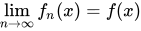
![{\displaystyle g_{n}:]0,1[\to \mathbb {R} ,x\mapsto f_{n}(x)-f(x)}](https://wikimedia.org/api/rest_v1/media/math/render/svg/fc6dfe3ef520685da246bf3d9512545f354ca73a)


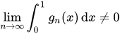


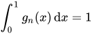
![{\displaystyle x\in ]0,1[\setminus ]0,{\tfrac {1}{2^{n}}}[}](https://wikimedia.org/api/rest_v1/media/math/render/svg/4fb817e391965001ad516777fc37a713167e4b42)


![{\displaystyle ]0,{\tfrac {1}{2^{n}}}[}](https://wikimedia.org/api/rest_v1/media/math/render/svg/230c5da1171460d523541d35b417d9c4c539768f)

![{\displaystyle x\in ]0,{\tfrac {1}{2^{n}}}[}](https://wikimedia.org/api/rest_v1/media/math/render/svg/4ae07e18712516f4e648494927b5bddc95be56d6)

![{\displaystyle g_{n}:]0,1[\to \mathbb {R} ,x\mapsto {\begin{cases}0&{\text{für }}x\in [{\tfrac {1}{2^{n}}},1[\\2^{n}&{\text{für }}x\in ]0,{\tfrac {1}{2^{n}}}[\end{cases}}}](https://wikimedia.org/api/rest_v1/media/math/render/svg/8bb1aadbdc59c4167f5a2ef0e5f059df91a43797)


